Code
fib_func <- function(N = ___, init = ___) {
    ...
    return(fib)
}x_recycled <- rep(x, length(y))[1:length(y)]).drop option when subsetting an array, matrix, or data frame! If the subsetting procedure selects only a single element, unless you use drop = FALSE, the result will be a length-one vector that “throws out” the other dimensions of your data structure. This can result in bugs if your code assumes that the result of the subset will have a consistent number of dimensions.The following set of R coding exercises are meant to prepare you for the kind of coding that will be involved in writing our first cognitive model simulations. It is not exhaustive of all the things that you can do with R, but it addresses many of the essentials. It also exemplifies the workflow involved in building a model:
These exercises are based on everyone’s favorite sequence, the Fibonnacci sequence. The sequence is defined by a simple rule: the next value in the sequence is the sum of the previous two values. Written in Math, that’s: \[ f[i] = f[i - 2] + f[i - 1] \] where \(f[\cdot]\) is a value in the Fibonnacci sequence and \(i\) is the index of the next value. To get this sequence going, we need to know the first two values, \(f[1]\) and \(f[2]\). Typically, these are both set to 1. As a result, the beginning of the Fibonnacci sequence goes like this: \[ 1, 1, 2, 3, 5, 8, 13, \ldots \]
Anyway, let’s begin!
Write two versions of a chunk of code that will create a vector called fib that contains the first 20 values in the Fibonnacci sequence. Assume that the first two values in the sequence are 1 and 1. Write one version of the code that creates the vector by appending each new value to the end of fib. Write another version that assigns values to the corresponding entries in fib directly using the appropriate index (for this second version, you may want to use the rep function to create the fib vector).
Based on the code you wrote for the previous exercise, write a function that returns a vector containing the first N terms of the Fibonnacci sequence. Your function should take two arguments, the value N and a vector called init that contains the first two values in the sequence. Give those arguments sensible default values. The chunk below gives a sense of the overall structure your function should have:
fib_func <- function(N = ___, init = ___) {
...
return(fib)
}Write code that calls the function you wrote in the previous exercise several times, each time using a different value for the second value in the init argument (but the same value for N and for init[1]). Collect the results from each function call in a single data frame or tibble. The data frame or tibble should have a column that stores the second initial value, a column for the vector returned from the function, and a third column that is the value’s index within the sequence. An example of the kind of result you’re looking for is given below:
# A tibble: 8 × 3
  init2   fib     i
  <dbl> <dbl> <int>
1     1     1     1
2     1     1     2
3     1     2     3
4     1     3     4
5     4     1     1
6     4     4     2
7     4     5     3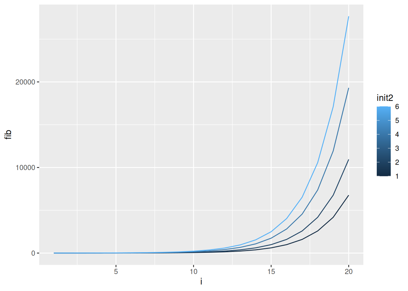
8 4 9 4Write code that uses the ggplot2 library to plot the values of the Fibonnacci sequence on the y-axis against their position in the sequence on the x-axis. Distinguish between different init2 values by using different colored lines. The result should look something like the plot below.
Write a new function that takes a third argument, n_back, which specifies how many of the previous values to add up to create the next value in the sequence. For the Fibonnacci sequence, n_back = 2, but in principle we could define other kinds of sequences too. Adapt the code you wrote for your previous exercises to explore what happens with different values of n_back. You may also want to include some code at the beginning of your function that checks to ensure that the number of initial values provided in the init argument is sufficient!