In the previous chapter, we saw several different examples of how computational cognitive models can represent the sorts of things we do cognition about: words, concepts, objects, events, etc. The representations were treated as given, either from a statistical procedure like Multidimensional Scaling or machine learning or from our own knowledge/expertise regarding the physical and conceptual features of items (like color, size, shape, etc.). Although one can view storage of new exemplars in memory as a kind of learning (see the Exercises), this chapter focuses on the kind of associative learning that is thought to underlie a variety of phenomena in cognition. Associative learning refers to the formation of functional links/connections/associations between elements that frequently co-occur. This form of learning is important for learning how words and referents go together, what properties objects have, and how to make predictions about what may happen next.
An important distinction in this form of learning is between supervised and unsupervised learning. In unsupervised learning, the learner does not have an explicit goal; as such, unsupervised learning often amounts to forming a representation of the patterns of correlation between elements in the learner’s environment. In supervised learning, the learner has a particular goal they are trying to achieve; in supervised learning, the learner gets feedback either from a “teacher” or from the environment itself about how well they achieved their goal. In supervised learning, the learner tries to form a representation that minimizes their “error”, that is, the discrepancy between the learner’s goal and the feedback they received.
The representations we explored in the last chapter all took the form of vectors which characterized the properties of items that someone might encounter. Since associative learning involves learning how properties go with one another, we will introduce another type of representation in this chapter: A matrix of associative weights. All the forms of learning we will examine in this chapter amount to making adjustments to the entries in one or more of these matrices. We’ll first see how this principle plays out in the context of a simple but powerful form of unsupervised learning: Hebbian learning.
11.1 Hebbian learning
Although this form of learning takes its name from Hebb (1949), the basic idea has been around since at least the ancient Greeks. The idea is that things that are experienced at the same time become associated with one another. Eventually, experiencing one thing “activates” or “evokes” or “retrieves” other things that were frequently encountered alongside it. In more recent times, the principle has been applied to neurons, giving rise to the dictum that “neurons that fire together wire together”.
To model Hebbian learning, we assume that the learner experiences discrete learning “events”. These “events” are analogous to the kinds of memory traces we used in the EBRW: each event is represented as a vector with \(D\) dimensions. These representations can be localist or either separable or integral distributed. Learning is modeled by making adjustments in a \(D \times D\) matrix, where the entry in the \(i\)th row and \(j\)th column is the associative weight between element \(i\) and element \(j\) of the event representations. These weights get updated each time an event occurs. As a result, the weights eventually come to represent the ways that different event element co-vary with one another.
11.1.1 Representing learning events
Let’s make this concrete by thinking back to the Blast cell example. Recall that those data involved participants with varying degrees of expertise in identifying whether a cell was a potentially cancerous “blast” cell or not, just by looking at a picture of the cell. Let’s imagine a related but somewhat simpler scenario, based on those used by Medin et al. (1982), that puts us in the position of being a novice gradually learning to become an expert.
Imagine that we are new doctors reading case reports that describe the presence or absence of four symptoms in each patient. For the moment, we are only interested in how these different symptoms may or may not co-vary with one another. The four symptoms are swollen eyelids, splotchy ears, discolored gums, and nosebleed. We have eight patient reports, and we can represent each report using a separable distributed vector with \(D = 4\) dimensions. As shown below, we can represent the presence of a symptom with a 1 and its absence with a 0.
Before reading any of the patient reports, we are a tabula rasa, a “blank slate”. That means we don’t know anything about how any of the symptoms go together. This state of initial ignorance is represented by an associative weight matrix that is filled with zeros. This is illustrated below.
How should we update our matrix of associative weights on the basis of this report? Since discolored gums and nosebleed were both present, we should increment the cells of the matrix corresponding to the combination of those symptoms. Moreover, since discolored gums and nosebleed are both present with themselves, we might as well update those cells of the matrix too. The result is that our new matrix might look something like this:
To formalize what we just did, we will draw on one concept we have already seen and another concept we’ve sort of seen, if through a glass darkly. For the concept we have seen, recall that our models of choice and response time involved accumulating samples of evidence, where we added the new sample to a “running total”. That’s exactly how we will be updating our matrix of associative weights, and we can write it formally like this: \[
W(t + 1) = W(t) + \Delta W(t)
\] where \(W(t)\) is our matrix of associative weights at the current time (\(t\)), \(W(t + 1)\) is our updated matrix after experiencing the learning event that occurs at time \(t\), and \(\Delta W(t)\) is how we change our weights on the basis of the learning event experienced at time \(t\). This is just like accumulating samples of evidence, but instead we are accumulating changes in associative weights over time.
Now for the thing we haven’t exactly seen, at least not in this form: Where do we get \(\Delta W(t)\)? Since we are talking about adding something to a \(D \times D\) matrix, we already know that \(\Delta W(t)\) must also be a \(D \times D\) matrix. We also know conceptually what \(\Delta W(t)\) needs to do: It needs to represent the combinations of features that were present in the learning event at time \(t\). Recall from last chapter that, when dealing with binary 0/1 vectors, the dot product between two such vectors gave us a count of the number of features that were present (i.e., coded as 1) in each representation. This is because when \(x_{ik} = 1\) and \(x_{jk} = 1\), \(x_{ik} x_{jk} = 1\), otherwise \(x_{ik} x_{jk} = 0\). This is the idea behind what we are about to do.
We can get \(\Delta W(t)\) by taking the outer product of the learning event representation \(\mathbf{x}(t)\) with itself. The outer product between two vectors \(\mathbf{a}\) and \(\mathbf{b}\) is sometimes written \(\mathbf{a} \otimes \mathbf{b}\). If \(\mathbf{a}\) has length \(N\) and \(\mathbf{b}\) has length \(M\), then \(\mathbf{a} \otimes \mathbf{b}\) is an \(N \times M\)matrix where the entry in the \(i\)th row and \(j\)th column is the product between the \(i\)th element of \(\mathbf{a}\) and the \(j\)th element of \(\mathbf{b}\). This is illustrated in the example below, showing that the outer function in R gives us the outer product.
Code
a <-c(1, 0, 0, 1)b <-c(1, 0, 1)# Outer product of a and bouter(a, b)
So if the vector \(\mathbf{x}(t)\) represents the learning event experienced at time \(t\), then \[
\Delta W(t) = \lambda \left[ \mathbf{x}(t) \otimes \mathbf{x}(t) \right]
\] where \(\lambda\) is a parameter that represents the \(learning rate\). In the present example, we will keep things simple and assume \(\lambda = 1\), but we will make use of this parameter later.
Getting back to our symptom example, we can write the update procedure in R like this:
You might already anticipate where we are going: We can use a for loop to update the matrix of associative weights for each learning “event”, i.e., for each patient record we read.
Code
# Initialize weights to zeroassc_weights <-matrix(0, nrow =ncol(event), ncol =ncol(event))# Specify learning ratelearning_rate <-1# Update weights for each eventfor (i in1:nrow(event)) { assc_weights <- assc_weights + learning_rate *outer(event[i,], event[i,])}knitr::kable(assc_weights)
swollen_eyelids
splotchy_ears
discolored_gums
nosebleed
swollen_eyelids
5
3
3
3
splotchy_ears
3
5
3
3
discolored_gums
3
3
5
5
nosebleed
3
3
5
5
11.1.3 Using what you’ve learned
Via Hebbian learning, we have accumulated information about the co-occurrence patterns of different features (symptoms) across a series of learning events (patient records). We can use the resulting matrix of associative weights to do something that has been labeled in a few ways, such as cued recall, pattern completion, inference, and fill-in-the-blanks. The idea is that if we know that a patient has some symptoms, we can use the matrix of associative weights to make a reasonable guess about whether they have other symptoms, based on the degree to which those other symptoms co-occurred with the ones we know about. As the various names listed above imply, this is the same kind of process that goes on when we, say, correctly infer that penguins have wings by knowing that they have beaks and webbed feet (we might also incorrectly infer that penguins can fly for the same reason!).
Say, for example, that we know a patient has discolored gums. By looking at the corresponding row in our matrix of associative weights, we can see that this symptom co-occurs with nosebleed more often than it does with either swollen eyelids or splotchy ears, as shown below.
Of course, the entries in our associative weight matrix are just numbers, they are not behavior. We need an additional process that enables us to predict behavior on the basis of the knowledge represented by the associative weight matrix. The relevant behavior here is whether or not you would be willing to say that a patient had symptom \(k\)—this is a choice. We could also model the response time associated with that choice (see the Exercises), but for now we only focus on choice behavior.
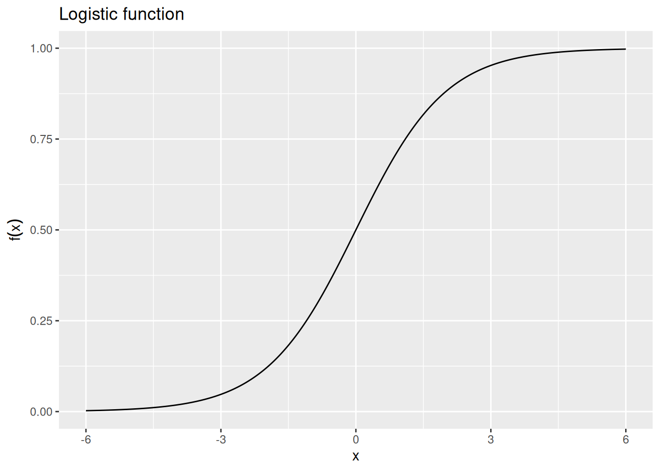
Specifically, we will transform the numbers extracted from the associative weight matrix into probabilities using the logistic function. This function will be familiar if you’ve done logistic regression, since it transforms unrestricted real numbers into the range between zero and one. The formula for the logistic function is \[
f(x) = \frac{1}{1 + \exp \left(-x \right)}
\] and it looks like this:
Code
tibble(x =seq(-6, 6, length.out =501)) %>%mutate(y =1/ (1+exp(-x))) %>%ggplot(aes(x = x, y = y)) +geom_line() +labs(x ="x", y =expression(f(x)), title ="Logistic function")
As shown above, the logistic function returns values greater than 0.5 whenever its argument \(x\) is a positive number. When \(x\) is negative, the logistic function returns values less than 0.5. And if \(x = 0\), the logistic function is exactly 0.5.
We can apply the logistic function to the row of the associative weight matrix above:
Of course, we can probably ignore the entry for discolored_gums because we already know the patient has those! Looking at the other probabilities, they are pretty big, reflecting the fact that the associative weights are also pretty large. The magnitude of the weights depends on the learning rate parameter. The chunk of code below shows what happens if we reduce the learning rate.
Code
# Initialize weights to zeroassc_weights <-matrix(0, nrow =ncol(event), ncol =ncol(event))# Specify learning ratelearning_rate <-0.2# Update weights for each eventfor (i in1:nrow(event)) { assc_weights <- assc_weights + learning_rate *outer(event[i,], event[i,])}knitr::kable(assc_weights)
With a smaller learning rate, the probabilities are not so extreme, and there is a bigger difference between the larger probabilities and smaller probabilities. Even so, we can anticipate that more learning will cause these weights to keep increasing and the probabilities to increase along with them. How can we address this counterintuitive behavior?
11.1.4 Discriminative learning
The fault, as it turns out, is not in our stars but in our representations. Recall that we coded the presence/absence of symptoms as 1 or 0. As a result, associative weights can only ever increase with learning. To avoid this, we can instead code the absence of a symptom as -1. By using negative values, we can represent the absence of a feature more explicitly, thereby allowing us to learn to discriminate between the presence or absence of different features.
First, let’s see what our learning event representations look like now:
We can see that the fact that discolored gums and nosebleed were both present while swollen eyelids and splotchy ears were not will result in a lowering of the associative weight between those two sets of symptoms.
Now let’s see what the final set of associative weights looks like:
Code
# Initialize weights to zeroassc_weights <-matrix(0, nrow =ncol(event), ncol =ncol(event))# Specify learning ratelearning_rate <-1# Update weights for each eventfor (i in1:nrow(event)) { assc_weights <- assc_weights + learning_rate *outer(event[i,], event[i,])}knitr::kable(assc_weights)
swollen_eyelids
splotchy_ears
discolored_gums
nosebleed
swollen_eyelids
8
0
0
0
splotchy_ears
0
8
0
0
discolored_gums
0
0
8
8
nosebleed
0
0
8
8
Now if we know a patient has discolored gums, we are very sure that they also have nosebleed and are equivocal about whether or not they have swollen eyelids or splotchy ears, as shown below:
On the other hand, if we know a patient has swollen eyelids, we don’t have any strong opinions about whether or not they have any other symptoms (though we think it is more likely than not). Note that this is a consequence of the fact that discolored gums and nosebleed did tend to co-occur in our training events, whereas swollen eyelids did not systematically covary with any other symptoms.
So far, we have only thought about situations in which a single symptom was given for a new patient. What if we know that a patient has 2 symptoms or 3? Or what if we know they do not have a particular symptom? To address these situations, we need to go beyond just looking at a single row at a time.
To appreciate what we are about to do, imagine that we knew a patient had discolored gums and that they did not have swollen eyelids. In that case, the strength of support for each feature would be the row corresponding to discolored_gumsminus the row corresponding to swollen_eyelids, as shown below:
When we apply the logistic function to the vector above, we are still equivocal about splotchy ears but we are actually more sure that they have nosebleed:
We can make the logic of what we just did to obtain that prediction more general. We will again make use of some linear algebra. Specifically, we will obtain the “strength of support” for each symptom by multiplying the matrix of associative weights with a vector that encodes the presence/absence/missingness of each known symptom. This vector is called a “probe” or a “cue”, and the result will be another vector that gives the total degree of support for each symptom. In math, we can write the operation like this: \[
\mathbf{o} = \mathbf{c} W
\] where \(\mathbf{c}\) is the cue (or probe) vector and \(\mathbf{o}\) is the “output” vector.
The example above corresponds to the following cue vector:
Notice that we use -1 to code for the known absence of a feature, 1 to code for the known presence of a feature, and 0 to code for “missing knowledge” about a feature.
We can use the cue vector to “probe” the associative weight matrix. In R, matrix multiplication uses the %*% operator (think of it as a “fancy multiplication”). So the code below directly implements the equation listed above:
And as we hoped, we get the same result from our fancy linear algebra as we did when we did it by hand earlier. The point of introducing this linear algebra now is that it will generalize more readily to situations in which we have more complex event representations (e.g., integral representations).
11.1.6 Associating events with actions
In the preceding examples, the learner associated features of events with one another, but now we consider how to model learning the relations between features of events and outcomes or actions. In the context of our ongoing medical example, imagine that a new doctor is learning to diagnose whether or not someone has a particular disease based on the pattern of symptoms they display. Now, instead of associating symptoms with symptoms, the doctor needs to associate symptoms with the presence/absence of the disease. Modeling this form of learning will require making two changes to the Hebbian learning model we have been building so far.
First, we need to redefine the associative weight matrix \(W\). Before, it was \(D \times D\), where \(D\) is the number of dimensions in our learning event representations. Now, it will be \(D \times O\), where \(O\) is the number of dimensions used to represent the available actions. Sometimes, as in some of the examples below, \(O\) will equal 1 if the learner just needs to decide whether to take an action or not (e.g., whether or not someone has a disease). But in general, \(O\) could have many dimensions if the learner can take many actions or if the actions are sufficiently complex that they require a distributed representation. The entry in the \(i\)th row and \(j\)th column of our new associative weight matrix will represent the strength of association between event dimension \(i\) and action/outcome dimension \(j\).
The other thing we need to do is define, for each learning event, the “label” or “correct answer” that is associated with it. In the model implementation below, we do this by having two matrices: an event matrix that stores the features of each learning event, with one row per event and one column per feature; and a target matrix that stores the “correct answer” for each event, with one row per event and one column per outcome dimension.
The example below uses the same set of symptoms as our running example. The first four patients were diagnosed with a disease while the second four were not.
In the end, the new doctor has learned that swollen eyelids are strongly diagnostic of the disease, splotchy ears are weakly diagnostic, discolored gums are weakly counter-indicative of the disease, and nosebleed is uninformative.
Notice that all we needed to do to model this form of associative learning was to swap out event for target. Formally, we can specify the learning procedure like this: \[
\Delta W(t) = \lambda \left[ \mathbf{x}(t) \otimes \mathbf{t}(t) \right]
\] where \(\lambda\) and \(\mathbf{x}(t)\) are as defined above and \(\mathbf{t}(t)\) is the vector representation of the target (“correct answer”) for the learning event experienced at time \(t\).
11.2 Error-driven learning
As noted above, Hebbian learning—whether of associations between event features or associations between events and actions—was a form of unsupervised learning, since the learner had no explicit goal other than to learn. In supervised learning, a learner again associates features of events with different actions or outcomes. The difference between supervised and unsupervised learning is that, in supervised learning, the adjustments the learner makes to their matrix of associations depends on the error between the target action/outcome and the learner’s guess or prediction about the action/outcome. Each time a learning event occurs, the learner uses the features of that event to form a representation of the action/outcome they select. The learner then receives feedback telling them the correct action/outcome they should have chosen. The goal of the learner is to adjust their associative weights in such a way that they reduce the discrepancy between the action/outcome they pick and the one they are told is correct.
To return to our running example, in supervised learning, the new doctor examines the symptoms of a patient report (this is the “learning event”), makes a diagnosis (this is the chosen action/outcome), and then gets told what the correct diagnosis would have been for that patient (this is the feedback). The new doctor then has to adjust the pattern of associations between symptoms (learning event features) and diagnoses (actions/outcomes).
We can imagine the same kind of learning occurring in many situations: When you are learning language, you might choose which word to use to describe an object based on its visible features (e.g., calling a black and white creature with four legs a “zebra”) and then someone nearby would either confirm your choice or provide the correct name (e.g., “no, that’s a dalmatian”). When you are learning a skill like using a tool or playing an instrument, you take an action (e.g., pressing a key on a keyboard) and then get feedback about whether it was correct or not (e.g., you hear the correct note you should have played).
Formally, error-driven learning happens in two steps: \[\begin{align*}
\mathbf{y}(t) & = f \left[ \mathbf{x}(t) W(t) \right] & \text{Make a prediction/guess} \\
\Delta W(t) & = \lambda \left\lbrace \mathbf{x}(t) \otimes \overbrace{\left[\mathbf{t}(t) - \mathbf{y}(t) \right]}^{\text{Error}} \right\rbrace & \text{Adjust weights in proportion to error}
\end{align*}\]
You may notice the mysterious function \(f\) in the first line above. This is because sometimes our prediction is a function of the associative weights and event features, like we saw with the logistic function above. Indeed, the logistic function is a common choice for \(f\) because we are often interested in modeling learning where the outcome is a binary decision (e.g., approach/avoid, good/bad, diagnose or not, etc.).
11.2.1 Of salivating dogs and doctors
The error-driven learning rule written above is a kind of Delta rule originally proposed by Widrow & Hoff (1960) but applied to animal and human learning by Rescorla & Wagner (1972). In particular, Rescorla & Wagner (1972) showed how error-driven learning could explain various phenomena in classical conditioning, hence the reference in the section title to Pavlov’s salivating dogs.
Conditioning experiments are functionally identical to the disease diagnosis example, along with many other cases in which a learner needs to form a prediction or expectation on the basis of the features of some event.
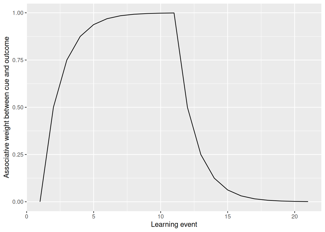
The code below illustrates how error-driven learning can explain extinction. We imagine that a single cue is presented for n_early times at the beginning of the experiment, when it is paired with the presence of some outcome. After that, we present the same cue again for n_late trials, but now it is no longer paired with the outcome. These patterns are built into the event and target matrices below. In addition, because the prediction is about the presence/absence of the outcome, the function \(f\) above is the logistic function.
You’ll notice too that this code stores the associative weights on each trial in an array. We can then use the array2DF function to make a pretty plot of how the associative weights change from one learning event to the next.
As we can see, the associative weight between the cue and outcome increases at first, eventually saturating when the presence of the outcome is correctly predicted by the presence of the cue. When the outcome stops happening, now that prediction is wrong and the associative weight diminishes in response, eventually returning to near zero.
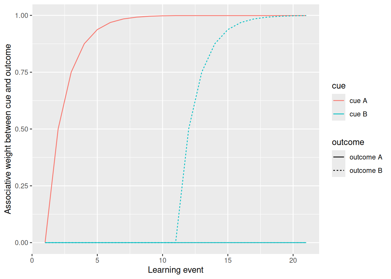
The next example of the Rescorla & Wagner (1972) model in action illustrates learning two different associations, one between an early cue and an early outcome and another between a late cue and a late outcome. Since associative weights only change in order to reduce error, the early-learned weights are preserved through the later phase of learning.
The following is a more complex learning situation known as a blocking paradigm (Kruschke, 2011). In the early phase, outcome A is paired with cue A and outcome B is paired with cue E. During the later phase, outcome A is paired with both cue A and cue B while outcome B is paired with cues C and D. The question is: Does the fact that cue A and outcome A had already been paired in the early phase block learning of an association between cue B and outcome A? That question is addressed by presenting transfer trials to the learner, coded below in the matrix transfer_event.
The first transfer trial involves presenting cues B and D to the learner. If cue B had been blocked, the learner should have a stronger expectation that outcome B would occur over outcome A.
The second transfer trial involves presenting cues A and C to the learner. If cue B had been blocked, then cue A should remain a stronger predictor of outcome A relative to how strongly cue C predicts outcome B.
We can see that, according to the Rescorla & Wagner (1972) model, learning of the association between cue B and outcome A has indeed been “blocked”. The reason is because the previously learned association between cue A and outcome A means that there is simply no need to learn a new association between cue B and outcome A—the learner is already capable of predicting the correct outcome. The result is that, as predicted by blocking, the learner is more likely to predict outcome B in the first transfer trial and is more likely to predict outcome A in the second transfer trial.
11.2.2 Batch learning
Applying the Rescorla & Wagner (1972) model to our novice doctor presents a challenge, namely, that the order in which events are encountered is no longer relevant to the doctor, since they can read the reports in any order. To model this form of learning, instead of updating the matrix of associative weights after each event, we can accumulate the changes across all events and update them all at once. This is called batch learning because the learner experiences a batch of events. This is a common approach in neural network models, as we shall see below.
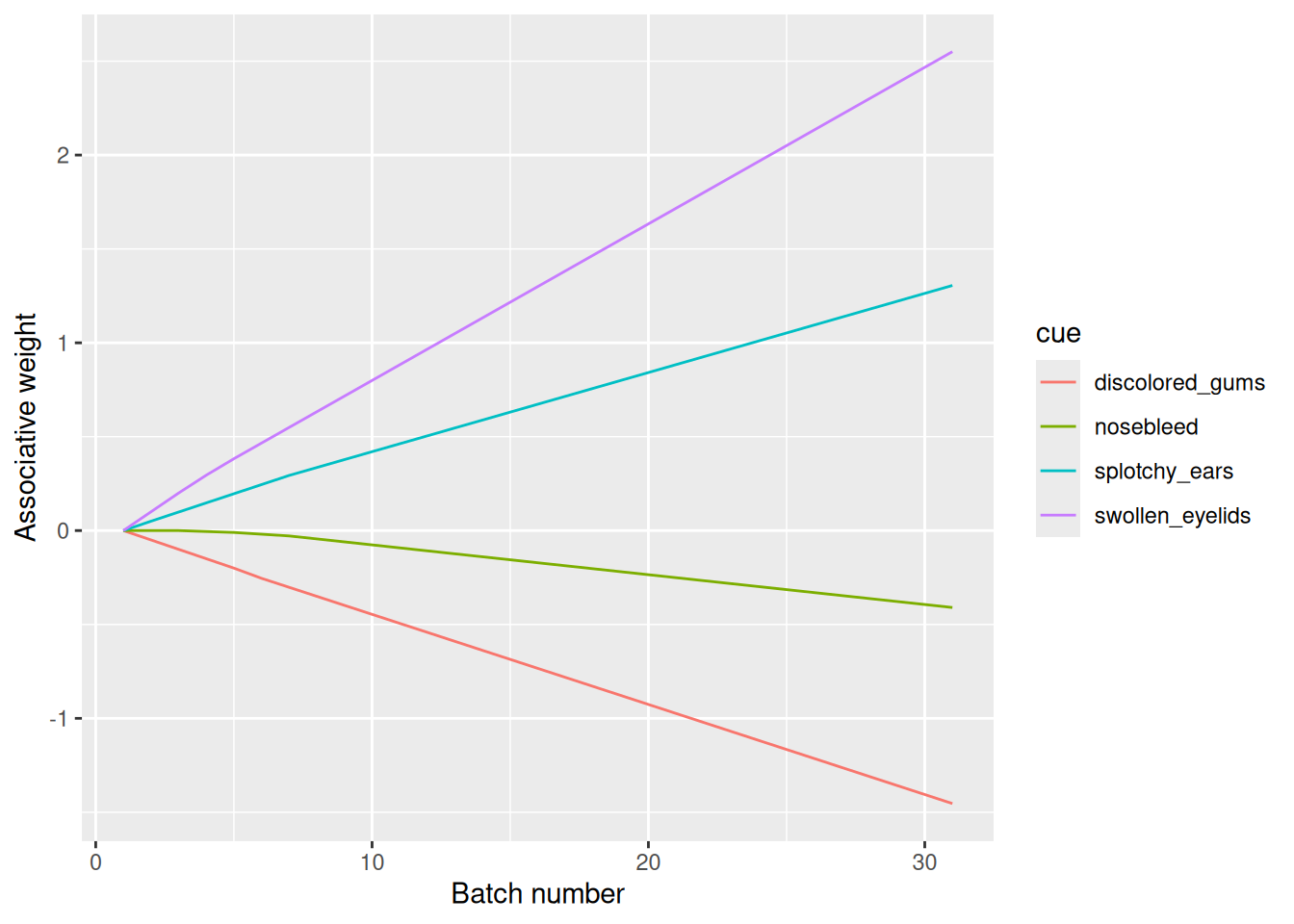
Batch learning is implemented in the chunk of code below, which also allows for the number of batches n_batch to be varied. Notice that error-driven learning can also achieve discriminative learning without needing to code event features as -1 and 1.
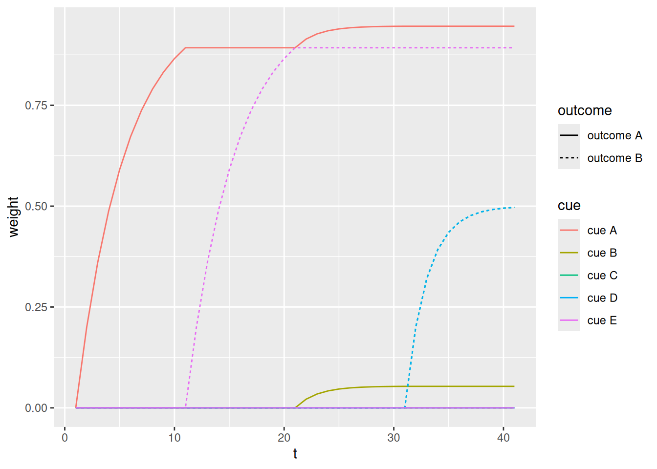
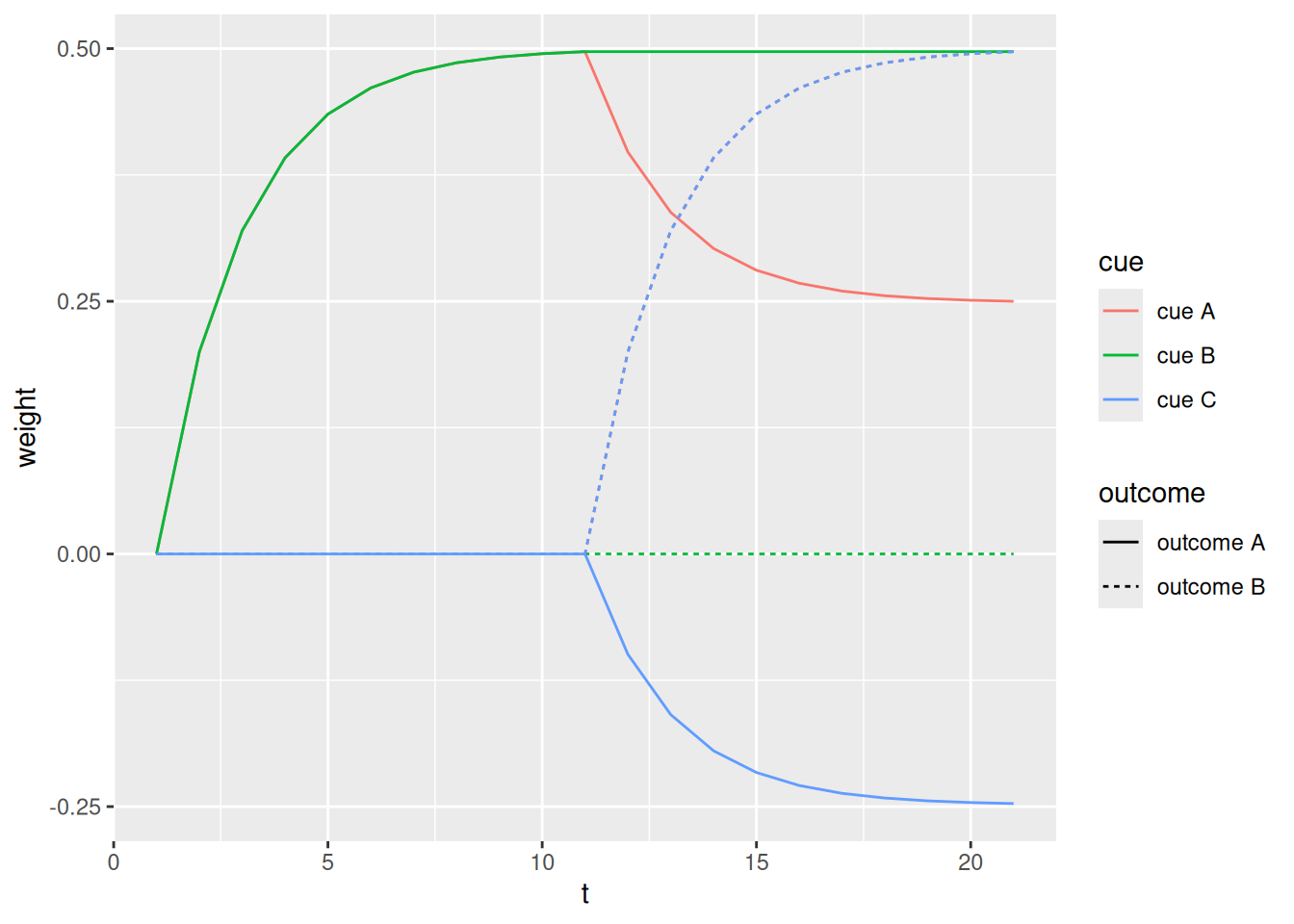
Since the Rescorla & Wagner (1972) model has been doing well so far, let’s present another learning situation to it. This situation is called highlighting(Kruschke, 2009) and, like blocking, involves an early and late set of learning events. In the early events, cues A and B are both paired with outcome A. In the late events, cues A and C are both paired with outcome B. The critical thing is that cue A is paired with both outcomes with equal frequency. If a learner were only sensitive to those frequencies, then cue A would be equally associated with both outcomes. Moreover, the learner would be ambivalent if presented with both cues B and C, since each had been paired with their respective outcomes an equal number of times. As you might guess, those two situations constitute the transfer_events in the code below.
However, animals, whether human or otherwise, do not show the pattern of results described above. In fact, learners tend to associate cue A with the early outcome more than the late outcome. And when confronted with both cues B and C, learners are more likely to expect the later outcome (outcome B) over the early one. This phenomenon is referred to as highlighting since the novelty of cue C, when it appears, seems to “highlight” it as the “true predictor” of outcome B. For the same reason, learners tend not to “unlearn” the early-learned association between cue A and outcome A.
Let’s see whether Rescorla & Wagner (1972) correctly predict this outcome…
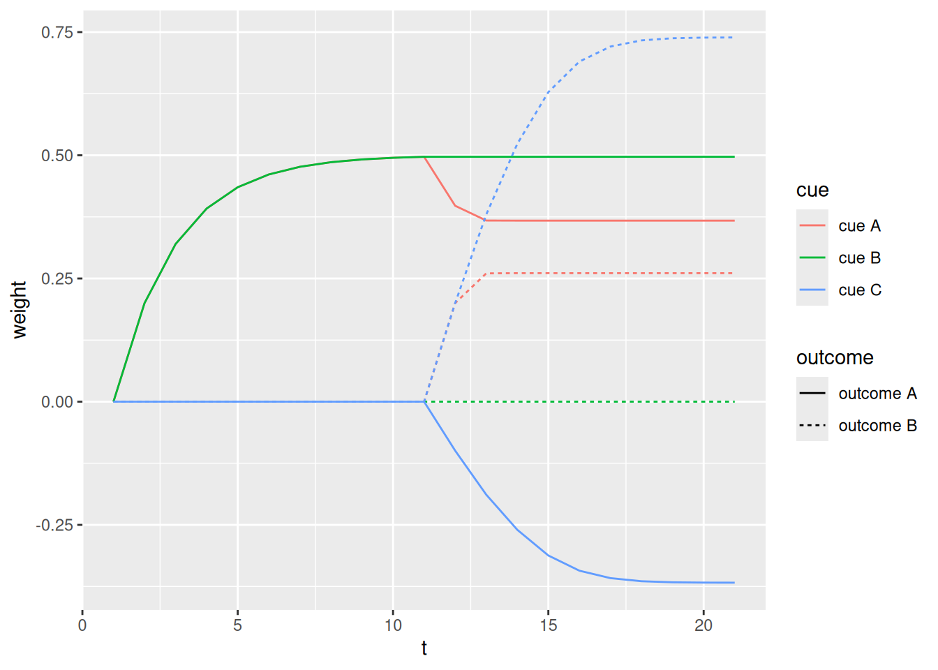
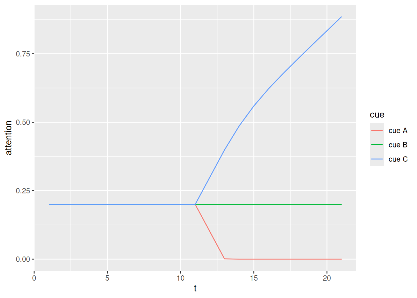
Unfortunately for Rescorla & Wagner (1972), their error-driven learning model cannot predict highlighting. To address this, Mackintosh (1975) suggested that the learning rates in the model may depend on the relative predictive strength of the available cues on each trial. This is a form of selective attention, in that it predicts that attention will be drawn to cues that do not yet have any strong associations. In other words, when the second learning phase begins, attention is drawn to cue C because it has no strong associations whereas attention is drawn away from cue A, since it is already strongly associated with outcome A.
Formally, incorporating attention into error-driven learning involves introducing an associative weight on each cue which determines the learning rate on each event. In the code below, the associative weight for each cue is the sum of the corresponding row in the associative weight matrix. The attention weight on each cue is adjusted in proportion to the difference between its associative weight and the sum of the associative weights for the other cues present in the current event. Note that, in the model below, the learning_rate parameter refers to the rate at which attention weights are adjusted from one event to the next. These attention weights are, in turn, the degree to which associative weights are adjusted from one event to the next.
As we can see, incorporating a role for attention produces the highlighting effect. When cue C appears, the attention weight on cue A rapidly diminishes, such that its association with outcome A is preserved through the second half of learning. On the other hand, the extra attention devoted to the novel cue C means that its association with outcome B is stronger than the association between cue B and outcome A.
11.3 Exercises
Within the context of a model like the EBRW, storing a new exemplar as a trace in memory could be considered a form of learning, in the sense that the performance of the model changes as a function of having experienced that new exemplar. Compare and contrast this form of learning with the forms of learning we encountered in this chapter.
Describe how you would use the output of any of the learning models we’ve seen in this chapter to predict not only choice behavior, but also choice and response time.
Try running the two-cue-two-outcome Rescorla-Wagner model from earlier in the chapter, but instead of coding the events as c(1, 0) for the early cues and c(0, 1) for the later cues, try using c(-1, 1) for the later cues. Describe what happens to the associative weight between cue A and outcome B. Describe a situation that might produce similar learning trajectories.
In the chapter, we saw that one way to allocate attention to cues during learning is based on the idea that attention is attracted to cues which are not yet strongly associated to anything else. What other principles could govern how attention is allocated to different cues during learning?
Hebb, D. O. (1949). The organization of behavior: A neuropsychological theory. Wiley.
Kruschke, J. K. (2009). Highlighting: A canonical experiment. In Psychology of learning and motivation (Vol. 51, pp. 153–185). Elsevier.
Kruschke, J. K. (2011). Models of attentional learning. In E. M. Pothos & A. J. Wills (Eds.), Formal approaches in categorization (pp. 120–152). Cambridge University Press.
Mackintosh, N. J. (1975). A theory of attention: Variations in the associability of stimuli with reinforcement. Psychological Review, 82(4), 276–298.
Rescorla, R. A., & Wagner, A. R. (1972). A theory of Pavlovian conditioning: Variations in the effectiveness of reinforcement and nonreinforcement. In A. H. Black & W. F. Prokasy (Eds.), Classical conditioning II: Current research and theory (pp. 64–99). Appleton–Century–Crofts.
Widrow, B., & Hoff, M. E. (1960). Adaptive switching circuits. IREWESCON Convention Record, 96–104.