12 Learning useful representations
In the previous chapter, we looked at models that learned by adjusting a matrix of associative weights between two sets of nodes. In those models, knowledge was represented by the entries in that matrix, reflecting the degree to which event features would “activate” other nodes. We saw that one powerful form of learning was error-driven learning where weight adjustments were made explicitly for the purpose of reducing the error between the learner’s predictions/expectations and what actually transpired.
The models in this chapter also learn by attempting to minimize error and they also do so by adjusting entries in associative weight matrices. However, these models add a so-called “hidden layer” that intervenes between the event features that act as “input” and the predictions/expectations that act as “output”. This category of model was the core of the connectionist or parallel distributed processing (PDP) framework.
These models learn via an extended form of error-driven learning called backpropagation of error (Rumelhart et al., 1986). This learning procedure enables a model to learn how to form an internal representation of the events it encounters, in the form of a pattern of activation across the nodes of its “hidden layer”. Such representations are a form of integral distributed vector representation. The purpose of these representations is to re-encode the features of an event into a form that enables the model to make more correct predictions/actions.
The kinds of models we will see in this chapter can thus be viewed as psychological theories of how distributed vector representations are acquired via experience. As we have already seen these representations are themselves essential for understanding performance (choice and RT) in different cognitive tasks. So these models “peel back” one more layer of the cognitive onion to help us understand where those representations may have come from.
Unfortunately, as we shall see (and as was explicitly stated by the developers of these models), learning by backpropagation of error is not very biologically plausible. So while these models are often called “artificial neural networks”, the resemblance between them and real neurons should be viewed in only an abstract sense.
Another drawback with these models is that learning requires extensive experience before the associative weights in the network stabilize and stop getting adjusted. As a result, this form of learning should not be thought of as something that happens on short timescales. Indeed, it has been proposed by several authors that biological brains have two complementary learning systems (McClelland et al., 1995). There is a “fast” learning system—typically thought to depend on the hippocampus and other medial temporal lobe structures—that encodes distinct events as separate traces, like we saw with the EBRW. Meanwhile, there is also a “slow” learning system—typically thought to depend on cortical areas—that does the kind of gradual weight adjustment we will see in the models in this chapter. The fast learning system encodes separate traces for distinct events using distributed representations learned by the slow learning system.
12.1 Backpropagation of error
The models we will examine in this chapter all have the basic structure depicted in the graph below:
The circles represent the elements of different vector representations; each representation is referred to as a layer. The “i” nodes are elements of a vector that represents the “input”—this is a representation of a learning event, just like in the last chapter. The “o” nodes are elements of a vector that represents the action/prediction/expectation that the learner takes, again like we saw in the last chapter. The new thing are the “h” nodes, which represent the network’s internal (hidden) representation of the learning event.
The links between the nodes depict associative weights between them. In the previous chapter, we only had associative weights between “input” and “output”. In the models in this chapter, we consider two sets of associations represented by two matrices of associative weights. If there are \(D\) input dimensions, \(H\) hidden dimensions, and \(O\) output dimensions, we can write the matrix of weights from input to hidden as \(W_{ih}\) and the matrix of weights from hidden to output as \(W_{ho}\).
12.1.1 Forward propagation
Just like in the last chapter, we treat the pattern of activation on the output vector as a representation of what the learner expects or plans to do. The learner forms this representation by “propagating” the activity from the input layer to the hidden layer and then from the hidden layer to the output layer. Like last time, we can write that propagation process using some linear algebra: \[\begin{align} \mathbf{h} & = f_h \left( \mathbf{x} W_{ih} \right) & \text{Input to hidden} \\ \mathbf{o} & = f_o \left( \mathbf{h} W_{ho} \right) & \text{Hidden to output} \end{align}\] where \(\mathbf{x}\) is the vector representing the learning event, \(\mathbf{h}\) is the vector representing the pattern of activation at the hidden layer, and \(\mathbf{o}\) is the vector representing the pattern of activation at the output layer. Notice that we allow for the activity at the hidden and output layers to be functions of their corresponding “inputs”, indicated by \(f_h \left( \cdot \right)\) and \(f_o \left( \cdot \right)\). In this chapter, we will only look at models where both \(f_h\) and \(f_o\) are the logistic function we used last chapter, i.e., \[ f_h(a) = f_o(a) = \frac{1}{1 + \exp \left(-a \right)} \]
12.1.2 Backward propagation
The procedure above describes how the model forms an expectation \(\mathbf{o}\) on the basis of the event features \(\mathbf{x}\). As we saw last time, the vector \(\mathbf{o}\) can be treated as a vector of probabilities with which each output feature is expected to be present or not (since we are using the logistic function).
The model learns by first computing the error between its expectation and a “target” representation and then propagating that error signal backwards along the associative weights. That’s why this learning procedure is called “backward propagation”, or “backprop” for short (not to be confused with a lumbar support pillow).
To be more mathy about it, backprop essentially adds one step to the error-driven learning procedure we saw last time. The additional step is because we have to adjust two sets of associative weights, \(W_{ho}\) and \(W_{ih}\). The equations below spell out the process: \[\begin{align*} \mathbf{e_o} & = \mathbf{t} - \mathbf{o} & \text{Error between target and output} \\ \mathbf{d_o} & = \mathbf{e_o} \mathbf{o} \left(1 - \mathbf{o} \right) & \text{Derivative of error with respect to output activation} \\ \Delta W_{ho} & = \lambda_{ho} \left( \mathbf{h} \otimes \mathbf{d_o} \right) & \text{How much to adjust hidden to output weights} \\ \mathbf{d_h} & = W_{ho} \mathbf{e_o} \mathbf{h} \left(1 - \mathbf{h} \right) & \text{Derivative of error with respect to hidden activation} \\ \Delta W_{ih} & = \lambda_{ih} \left( \mathbf{x} \otimes \mathbf{d_h} \right) & \text{How much to adjust input to hidden weights} \end{align*}\] You may notice above some stuff about “derivatives”, but this is not so mysterious as at may first appear. We were able to avoid mentioning derivatives in the last chapter because we only needed to worry about how to adjust a single set of weights. But really what we were doing was computing how much the error would change if we adjusted each associative weight. That’s a derivative! Now that we have two sets of weights to learn, we need to consider how much each weight contributes to the total error at the output layer. Backprop just expands this concept of the derivative so that it can assign “blame” for the error to each weight.
You may notice the terms \(\mathbf{o} \left(1 - \mathbf{o} \right)\) and \(\mathbf{h} \left(1 - \mathbf{h} \right)\) in the derivative formulae above. That’s because we also need to consider the derivative of the link function for each layer. The derivative of the logistic function \(f \left( a \right)\), which we are using for both the hidden and output layers, is just \(f \left(a \right) \left[1 - f \left(a \right) \right]\), hence the appearance of those terms in the formulae above.
Finally, although we could use different learning rates for input-to-hidden and hidden-to-output weights, denoted \(\lambda_{ih}\) and \(\lambda_{ho}\) respectively, in the models below we will just use a single learning rate \(\lambda\) that applies to all weights.
12.1.3 Baseline activations
We will introduce one more aspect to these models that we did not employ earlier, which is the use of a “baseline” activity level for both the hidden and output layers. We can think of this baseline as like an intercept term in linear regression. And just like in linear regression, the intercept can be thought of as an “input” that has a constant value. These baseline levels will be learned just like the weights are, i.e., they will be adjusted so as to minimize error. Specifically, the learning rule is: \[\begin{align*} \Delta \mathbf{b_h} & = \lambda \mathbf{d_h} \\ \Delta \mathbf{b_o} & = \lambda \mathbf{d_o} \end{align*}\] where \(\mathbf{b_h}\) and \(\mathbf{b_o}\) are the baselines for the hidden and output units, respectively, and \(\mathbf{d_h}\) and \(\mathbf{d_o}\) are the vectors of error derivatives defined above.
12.2 Learning concept representations from properties
Now let’s see how one of these models works in a setting we have already seen. The example below shows how a simple backprop network can learn to represent the different concepts we saw in some of our preceding examples. Specifically, we will train the network to learn the features of different concepts. Each learning event will be represented with a localist vector representation of a concept. The output that the network will be trained to produce is a separable vector representation of the features of that concept. Thus, the network will learn to report the features of a concept, given the concept as a “cue”. We can think of this as like learning to provide a dictionary definition of a term.
What we are particularly interested in is the dynamics by which the network learns representations for the eight concepts. As we shall see, the representation that the network learns in its hidden layer will distinguish between broad categories early on and later come to make more fine-grained distinctions. This gradual differentiation over the course of learning is a natural consequence of error-driven learning: Since the biggest errors are due to the biggest confusions, those will be learned first.
Code
logistic_act <- function(x) {
    return(1 / (1 + exp(-x)))
}

# Localist representations of eight concepts
event <- matrix(c(
     1, 0, 0, 0, 0, 0, 0, 0,
     0, 1, 0, 0, 0, 0, 0, 0,
     0, 0, 1, 0, 0, 0, 0, 0,
     0, 0, 0, 1, 0, 0, 0, 0,
     0, 0, 0, 0, 1, 0, 0, 0,
     0, 0, 0, 0, 0, 1, 0, 0,
     0, 0, 0, 0, 0, 0, 1, 0,
     0, 0, 0, 0, 0, 0, 0, 1
), nrow = 8, ncol = 8, byrow = TRUE, dimnames = list(
    c("pine", "oak", "rose", "daisy", "robin", "canary", "sunfish", "salmon"),
    c("pine", "oak", "rose", "daisy", "robin", "canary", "sunfish", "salmon")
))

# Separable representations of concept features
target <- matrix(c(
     1, 0, 0, 0, 0, 1, 1, 1, 0, 0, 0, 0, 0, 0, 0, 0, 0, 1, 0, 0, 1, 1,
     0, 1, 0, 0, 0, 1, 1, 1, 0, 0, 0, 0, 0, 0, 0, 0, 0, 1, 0, 0, 1, 1,
     0, 0, 1, 0, 0, 0, 0, 0, 1, 1, 1, 0, 0, 0, 0, 0, 0, 1, 0, 0, 1, 1,
     0, 0, 0, 1, 0, 0, 0, 0, 1, 1, 1, 0, 0, 0, 0, 0, 0, 1, 0, 0, 1, 1,
     0, 0, 1, 0, 0, 0, 0, 0, 0, 0, 0, 1, 1, 1, 0, 0, 0, 0, 1, 1, 1, 1,
     0, 0, 0, 1, 1, 0, 0, 0, 0, 0, 0, 1, 1, 1, 0, 0, 0, 0, 1, 1, 1, 1,
     0, 0, 0, 1, 0, 0, 0, 0, 0, 0, 0, 0, 0, 0, 1, 1, 1, 0, 1, 1, 1, 1,
     0, 0, 1, 0, 0, 0, 0, 0, 0, 0, 0, 0, 0, 0, 1, 1, 1, 0, 1, 1, 1, 1
), nrow = 8, ncol = 22, byrow = TRUE, dimnames = list(
    c("pine", "oak", "rose", "daisy", "robin", "canary", "sunfish", "salmon"),
    c("is_green", "has_leaves", "is_red", "is_yellow", "can_sing", "has_bark", "is_big", "has_branches", "has_leaves", "has_petals", "is_pretty", "has_feathers", "can_fly", "has_wings", "has_scales", "can_swim", "has_gills", "has_roots", "can_move", "has_skin", "can_grow", "is_living")
))

learning_rate <- 0.05
n_hidden <- 6
n_epochs <- 5000
learn_by_epoch <- TRUE

n_hidden_snapshots <- 9
epoch_to_snap <- round(exp(seq(0, log(n_epochs), length.out = n_hidden_snapshots)))
snapshot_hidden_activation <- array(0, dim = c(n_hidden_snapshots, nrow(event), n_hidden), dimnames = list("epoch" = epoch_to_snap, "item" = rownames(event), "hidden_unit" = 1:n_hidden))

i_to_h_assc_weights <- matrix(rnorm(n = ncol(event) * n_hidden), nrow = ncol(event), ncol = n_hidden) * 0.01
h_to_o_assc_weights <- matrix(rnorm(n = n_hidden * ncol(target)), nrow = n_hidden, ncol = ncol(target)) * 0.01

hidden_baseline <- rnorm(n = n_hidden) * 0.01
output_baseline <- rnorm(n = ncol(target)) * 0.01

for (epoch in 1:n_epochs) {
    training_order <- sample(nrow(event))

    d_h_to_o <- 0 * h_to_o_assc_weights
    d_i_to_h <- 0 * i_to_h_assc_weights

    d_h_baseline <- 0 * hidden_baseline
    d_o_baseline <- 0 * output_baseline

    for (i in training_order) {
        # Forward propagation (prediction)

        # Note the use of `as.vector` to ensure result is a vector (not a matrix with a single row)
        hidden_activation <- logistic_act(as.vector(event[i,] %*% i_to_h_assc_weights) + hidden_baseline)
        output_activation <- logistic_act(as.vector(hidden_activation %*% h_to_o_assc_weights) + output_baseline)

        # Compute error at output layer
        output_error <- target[i,] - output_activation

        # Back propagation (learning)

        # Derivative of error with respect to output unit activation
        d_output_error <- output_error * output_activation * (1 - output_activation)

        # Derivative of error with respect to hidden unit activation
        d_hidden_error <- as.vector(h_to_o_assc_weights %*% d_output_error) * hidden_activation * (1 - hidden_activation)

        # How much to adjust the associative weights between the hidden and output layers
        d_h_to_o <- d_h_to_o + learning_rate * outer(hidden_activation, d_output_error)

        # How much to adjust the associative weights between the input and hidden layers
        d_i_to_h <- d_i_to_h + learning_rate * outer(event[i,], d_hidden_error)

        # How much to adjust the baseline of the output units
        d_o_baseline <- learning_rate * d_output_error

        # How much to adjust the baseline of the hidden units
        d_h_baseline <- learning_rate * d_hidden_error

        if (!learn_by_epoch) {
            # Adjust weights
            i_to_h_assc_weights <- i_to_h_assc_weights + d_i_to_h
            h_to_o_assc_weights <- h_to_o_assc_weights + d_h_to_o

            hidden_baseline <- hidden_baseline + d_h_baseline
            output_baseline <- output_baseline + d_o_baseline

            # Reset adjustment to zero
            d_h_to_o <- 0 * h_to_o_assc_weights
            d_i_to_h <- 0 * i_to_h_assc_weights

            d_h_baseline <- 0 * hidden_baseline
            d_o_baseline <- 0 * output_baseline
        }
    }

    if (learn_by_epoch) {
        # Adjust weights
        i_to_h_assc_weights <- i_to_h_assc_weights + d_i_to_h
        h_to_o_assc_weights <- h_to_o_assc_weights + d_h_to_o

        hidden_baseline <- hidden_baseline + d_h_baseline
        output_baseline <- output_baseline + d_o_baseline
    }

    if (epoch %in% as.numeric(dimnames(snapshot_hidden_activation)[[1]])) {
        for (i in 1:nrow(event)) {
            snapshot_hidden_activation[as.character(epoch), i, ] <- logistic_act(as.vector(event[i,] %*% i_to_h_assc_weights) + hidden_baseline)
        }
    }
}

array2DF(snapshot_hidden_activation) %>%
    mutate(item = factor(item, levels = rownames(event))) %>%
    mutate(hidden_unit = as.numeric(hidden_unit)) %>%
    mutate(epoch = factor(epoch, levels = as.character(sort(unique(as.numeric(epoch)))))) %>%
    ggplot(aes(x = hidden_unit, y = Value, color = item)) +
    geom_line() +
    scale_color_brewer(palette = "Paired") +
    facet_wrap("epoch", labeller = label_both)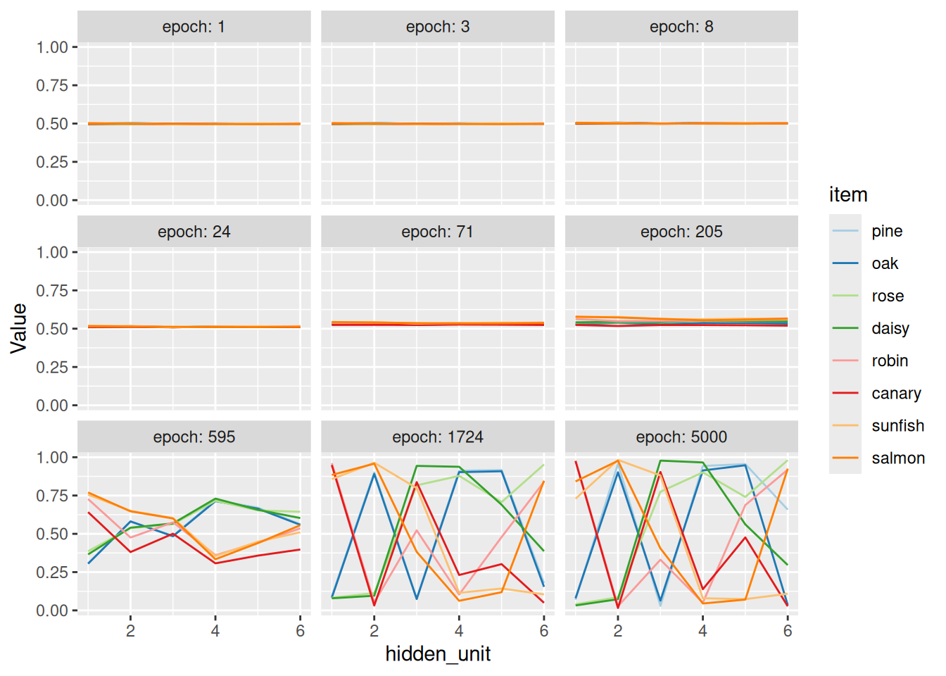
Code
item_mds <- array(0, dim = c(n_hidden_snapshots, nrow(event), 2), dimnames = list("epoch" = epoch_to_snap, "item" = rownames(event), "dim" = paste0("dim", 1:2)))

for (epoch in dimnames(snapshot_hidden_activation)[[1]]) {
    item_mds[epoch, , ] <- cmdscale(d = dist(snapshot_hidden_activation[epoch,,]), k = 2)
}

array2DF(item_mds) %>%
    pivot_wider(id_cols = c(epoch, item), names_from = dim, values_from = Value) %>%
    mutate(item = factor(item, levels = rownames(event))) %>%
    mutate(epoch = factor(epoch, levels = as.character(sort(unique(as.numeric(epoch)))))) %>%
    ggplot(aes(x = dim1, y = dim2, color = item)) +
    geom_path() +
    coord_equal() +
    scale_color_brewer(palette = "Paired") +
    labs(title = "Evolution of internal representations with learning", x = "Dimension 1", y = "Dimension 2", caption = "Visualization by multidimensional scaling")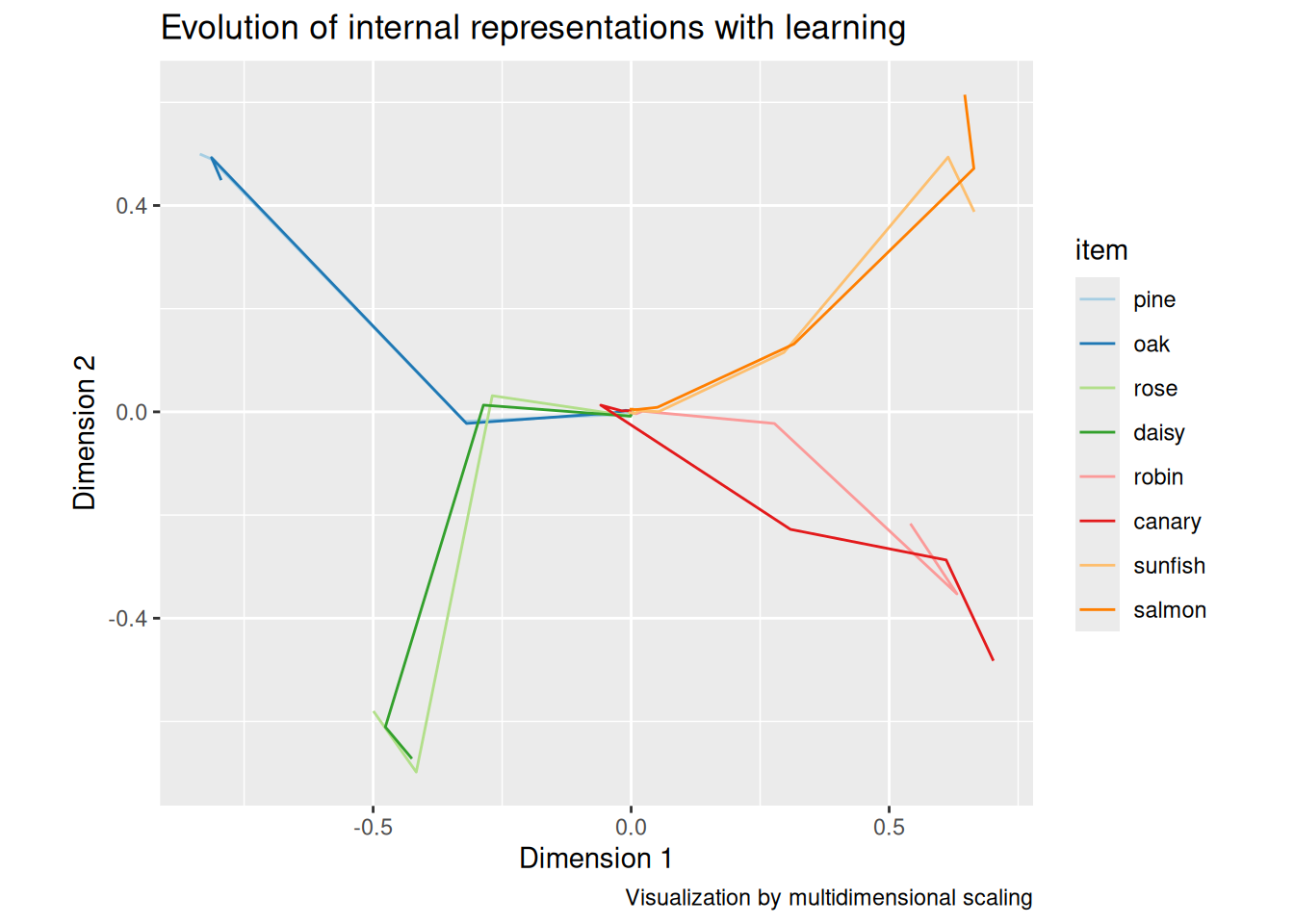
The model was trained in “batches”, like we saw last time, only those batches are referred to as “epochs”, following some rather grandiose terminology from the early days of such models. The code above takes “snapshots” of the hidden unit activations at various epochs during learning so we can examine gradual differentiation of the eight concepts. To get these snapshots, we cue the network with the vector representation of a concept and forward-propagate that activation into the hidden layer. The vector of activation values among the hidden units, \(\mathbf{h}\), is treated as a vector representation of that concept.
A common visualization technique in this domain is to use multidimensional scaling to plot the vector representations derived from the hidden layer in two dimensions. As you can see, the model learns first to distinguish animals and plants, then the subcategories of animals and plants, and finally individual animals within each subcategory. Again, this is a natural consequence of error-driven learning, but also mirrors the developmental trajectories by which many human learners acquire concepts (Rogers & McClelland, 2004).
Code
transfer_event <- event

transfer_hidden_activation <- matrix(0, nrow = nrow(transfer_event), ncol = n_hidden, dimnames = list(rownames(transfer_event), 1:n_hidden))
p_resp <- matrix(0, nrow = nrow(transfer_event), ncol = ncol(target), dimnames = list(rownames(transfer_event), colnames(target)))

for (i in 1:nrow(transfer_event)) {
    transfer_hidden_activation[i,] <- logistic_act(as.vector(transfer_event[i,] %*% i_to_h_assc_weights) + hidden_baseline)
    p_resp[i,] <- logistic_act(as.vector(transfer_hidden_activation[i,] %*% h_to_o_assc_weights) + output_baseline)
}

knitr::kable(p_resp)| is_green | has_leaves | is_red | is_yellow | can_sing | has_bark | is_big | has_branches | has_leaves | has_petals | is_pretty | has_feathers | can_fly | has_wings | has_scales | can_swim | has_gills | has_roots | can_move | has_skin | can_grow | is_living | |
|---|---|---|---|---|---|---|---|---|---|---|---|---|---|---|---|---|---|---|---|---|---|---|
| pine | 0.6197004 | 0.2152856 | 0.1634120 | 0.0023826 | 0.0000787 | 0.9250800 | 0.9248442 | 0.9249413 | 0.0654654 | 0.0653810 | 0.0655194 | 0.0003422 | 0.0003460 | 0.0003463 | 0.0290274 | 0.0291252 | 0.0290503 | 0.9841509 | 0.0158996 | 0.0159508 | 0.9934424 | 0.9934167 |
| oak | 0.3639541 | 0.7542412 | 0.0035378 | 0.0604771 | 0.0016651 | 0.9710283 | 0.9711196 | 0.9710512 | 0.0327099 | 0.0327668 | 0.0326952 | 0.0006676 | 0.0006763 | 0.0006762 | 0.0327475 | 0.0326825 | 0.0327317 | 0.9800315 | 0.0200837 | 0.0200627 | 0.9852742 | 0.9852162 |
| rose | 0.1171546 | 0.0051179 | 0.8592013 | 0.0786542 | 0.0023262 | 0.0339779 | 0.0337560 | 0.0338263 | 0.9526771 | 0.9526321 | 0.9527004 | 0.0370967 | 0.0370953 | 0.0370894 | 0.0009683 | 0.0009861 | 0.0009683 | 0.9703105 | 0.0296178 | 0.0296769 | 0.9930061 | 0.9930950 |
| daisy | 0.0253838 | 0.0450993 | 0.0555032 | 0.9082180 | 0.0622958 | 0.0514525 | 0.0517702 | 0.0516991 | 0.9389191 | 0.9389509 | 0.9388634 | 0.0445643 | 0.0445280 | 0.0445385 | 0.0015944 | 0.0016179 | 0.0015916 | 0.9610207 | 0.0388918 | 0.0388536 | 0.9854807 | 0.9857238 |
| robin | 0.0592497 | 0.0018862 | 0.9673368 | 0.0214734 | 0.0703603 | 0.0076952 | 0.0074745 | 0.0074523 | 0.0352395 | 0.0352719 | 0.0352792 | 0.9347017 | 0.9348090 | 0.9347979 | 0.0373993 | 0.0373436 | 0.0374353 | 0.0433034 | 0.9567807 | 0.9567997 | 0.9878454 | 0.9877362 |
| canary | 0.0026075 | 0.0145775 | 0.0436665 | 0.9792545 | 0.8833943 | 0.0039277 | 0.0039028 | 0.0038735 | 0.0438923 | 0.0439235 | 0.0438537 | 0.9448623 | 0.9447779 | 0.9447972 | 0.0529522 | 0.0529290 | 0.0529405 | 0.0255592 | 0.9744926 | 0.9743351 | 0.9806805 | 0.9806508 |
| sunfish | 0.0099680 | 0.0281456 | 0.0288670 | 0.9513678 | 0.0739919 | 0.0286904 | 0.0290737 | 0.0290171 | 0.0039767 | 0.0039643 | 0.0039774 | 0.0403594 | 0.0403262 | 0.0402801 | 0.9442030 | 0.9443196 | 0.9441888 | 0.0235738 | 0.9763927 | 0.9763234 | 0.9860802 | 0.9860688 |
| salmon | 0.1096960 | 0.0026860 | 0.9250481 | 0.0347728 | 0.0020557 | 0.0254518 | 0.0253029 | 0.0253500 | 0.0029490 | 0.0029360 | 0.0029553 | 0.0519291 | 0.0519060 | 0.0519225 | 0.9519660 | 0.9519600 | 0.9519801 | 0.0195692 | 0.9803492 | 0.9804679 | 0.9909340 | 0.9908830 |
Finally, the code above verifies that the model has, indeed, learned to correctly predict the features of each concept.
12.3 Autoencoders for learning co-occurrence patterns
Just like in the last chapter, backprop networks can learn to reproduce patterns. Such networks are called autoencoders. The only difference between the following example and the one above is that the target output is the same vector as the input. The value of backprop in this instance is that the network can learn a reduced representation that takes advantage of redundancies or patterns within the input vectors. This is conceptually similar to how principal components analysis works!
The example below uses the disease symptoms from last chapter. Notice that the last two symptoms, discolored gums and nosebleed, are correlated—they are either both present or both absent. Thus, even though the hidden layer only has 3 dimensions instead of 4, the model can correctly reproduce the pattern of symptoms for each patient.
Code
logistic_act <- function(x) {
    return(1 / (1 + exp(-x)))
}

event <- matrix(c(
    0, 0, 1, 1,
    1, 1, 1, 1,
    0, 1, 0, 0,
    1, 1, 1, 1,
    1, 0, 1, 1,
    1, 1, 0, 0,
    0, 1, 1, 1,
    1, 0, 0, 0
), nrow = 8, ncol = 4, byrow = TRUE,
dimnames = list(
    c("EM", "RM", "JJ", "LF", "AM", "JS", "ST", "SE"),
    c("swollen_eyelids", "splotchy_ears", "discolored_gums", "nosebleed")
))

target <- event

learning_rate <- 0.05
n_hidden <- 3
n_epochs <- 5000
learn_by_epoch <- TRUE

n_hidden_snapshots <- 9
epoch_to_snap <- round(exp(seq(0, log(n_epochs), length.out = n_hidden_snapshots)))
snapshot_hidden_activation <- array(0, dim = c(n_hidden_snapshots, nrow(event), n_hidden), dimnames = list("epoch" = epoch_to_snap, "item" = rownames(event), "hidden_unit" = 1:n_hidden))

i_to_h_assc_weights <- matrix(rnorm(n = ncol(event) * n_hidden), nrow = ncol(event), ncol = n_hidden) * 0.01
h_to_o_assc_weights <- matrix(rnorm(n = n_hidden * ncol(target)), nrow = n_hidden, ncol = ncol(target)) * 0.01

hidden_baseline <- rnorm(n = n_hidden) * 0.01
output_baseline <- rnorm(n = ncol(target)) * 0.01

for (epoch in 1:n_epochs) {
    training_order <- sample(nrow(event))

    d_h_to_o <- 0 * h_to_o_assc_weights
    d_i_to_h <- 0 * i_to_h_assc_weights

    d_h_baseline <- 0 * hidden_baseline
    d_o_baseline <- 0 * output_baseline

    for (i in training_order) {
        # Forward propagation (prediction)

        # Note the use of `as.vector` to ensure result is a vector (not a matrix with a single row)
        hidden_activation <- logistic_act(as.vector(event[i,] %*% i_to_h_assc_weights) + hidden_baseline)
        output_activation <- logistic_act(as.vector(hidden_activation %*% h_to_o_assc_weights) + output_baseline)

        # Compute error at output layer
        output_error <- target[i,] - output_activation

        # Back propagation (learning)

        # Derivative of error with respect to output unit activation
        d_output_error <- output_error * output_activation * (1 - output_activation)

        # Derivative of error with respect to hidden unit activation
        d_hidden_error <- as.vector(h_to_o_assc_weights %*% d_output_error) * hidden_activation * (1 - hidden_activation)

        # How much to adjust the associative weights between the hidden and output layers
        d_h_to_o <- d_h_to_o + learning_rate * outer(hidden_activation, d_output_error)

        # How much to adjust the associative weights between the input and hidden layers
        d_i_to_h <- d_i_to_h + learning_rate * outer(event[i,], d_hidden_error)

        # How much to adjust the baseline of the output units
        d_o_baseline <- learning_rate * d_output_error

        # How much to adjust the baseline of the hidden units
        d_h_baseline <- learning_rate * d_hidden_error

        if (!learn_by_epoch) {
            # Adjust weights
            i_to_h_assc_weights <- i_to_h_assc_weights + d_i_to_h
            h_to_o_assc_weights <- h_to_o_assc_weights + d_h_to_o

            hidden_baseline <- hidden_baseline + d_h_baseline
            output_baseline <- output_baseline + d_o_baseline

            # Reset adjustment to zero
            d_h_to_o <- 0 * h_to_o_assc_weights
            d_i_to_h <- 0 * i_to_h_assc_weights

            d_h_baseline <- 0 * hidden_baseline
            d_o_baseline <- 0 * output_baseline
        }
    }

    if (learn_by_epoch) {
        # Adjust weights
        i_to_h_assc_weights <- i_to_h_assc_weights + d_i_to_h
        h_to_o_assc_weights <- h_to_o_assc_weights + d_h_to_o

        hidden_baseline <- hidden_baseline + d_h_baseline
        output_baseline <- output_baseline + d_o_baseline
    }

    if (epoch %in% as.numeric(dimnames(snapshot_hidden_activation)[[1]])) {
        for (i in 1:nrow(event)) {
            snapshot_hidden_activation[as.character(epoch), i, ] <- logistic_act(as.vector(event[i,] %*% i_to_h_assc_weights) + hidden_baseline)
        }
    }
}

array2DF(snapshot_hidden_activation) %>%
    mutate(item = factor(item, levels = rownames(event))) %>%
    mutate(hidden_unit = as.numeric(hidden_unit)) %>%
    mutate(epoch = factor(epoch, levels = as.character(sort(unique(as.numeric(epoch)))))) %>%
    ggplot(aes(x = hidden_unit, y = Value, color = item)) +
    geom_line() +
    scale_color_okabeito() +
    facet_wrap("epoch", labeller = label_both)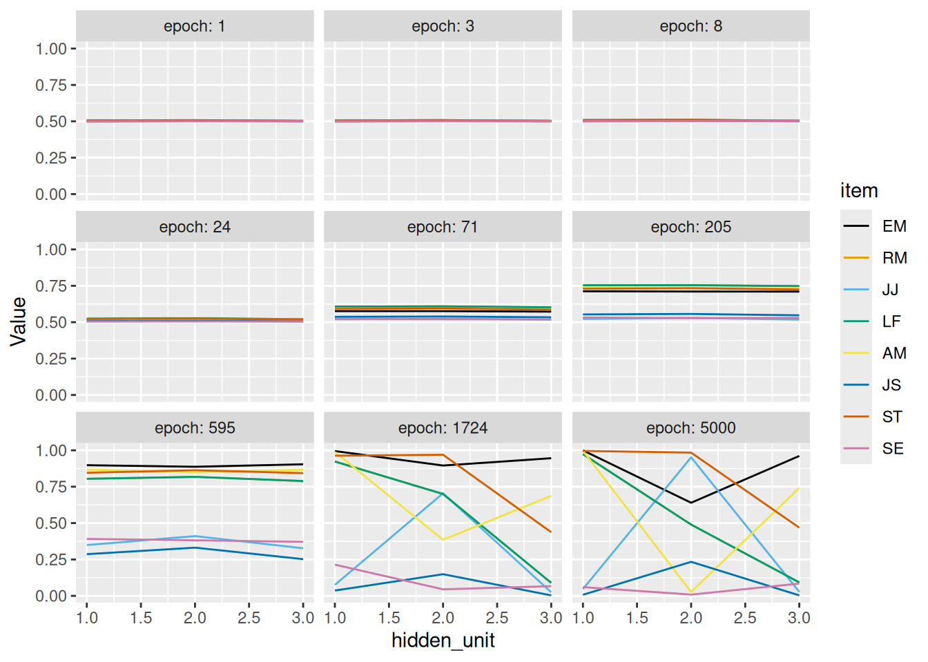
Code
item_mds <- array(0, dim = c(n_hidden_snapshots, nrow(event), 2), dimnames = list("epoch" = epoch_to_snap, "item" = rownames(event), "dim" = paste0("dim", 1:2)))

for (epoch in dimnames(snapshot_hidden_activation)[[1]]) {
    item_mds[epoch, , ] <- cmdscale(d = dist(snapshot_hidden_activation[epoch,,]), k = 2)
}

array2DF(item_mds) %>%
    pivot_wider(id_cols = c(epoch, item), names_from = dim, values_from = Value) %>%
    mutate(item = factor(item, levels = rownames(event))) %>%
    mutate(epoch = factor(epoch, levels = as.character(sort(unique(as.numeric(epoch)))))) %>%
    ggplot(aes(x = dim1, y = dim2, color = item)) +
    geom_path() +
    coord_equal() +
    scale_color_okabeito() +
    labs(title = "Evolution of internal representations with learning", x = "Dimension 1", y = "Dimension 2", caption = "Visualization by multidimensional scaling")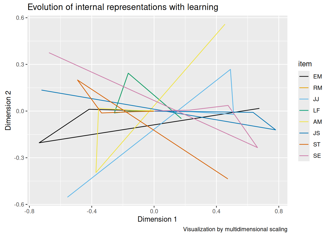
Code
transfer_event <- diag(ncol(event))
colnames(transfer_event) <- rownames(transfer_event) <- colnames(event)

transfer_hidden_activation <- matrix(0, nrow = nrow(transfer_event), ncol = n_hidden, dimnames = list(rownames(transfer_event), 1:n_hidden))
p_resp <- matrix(0, nrow = nrow(transfer_event), ncol = ncol(target), dimnames = list(rownames(transfer_event), colnames(target)))

for (i in 1:nrow(transfer_event)) {
    transfer_hidden_activation[i,] <- logistic_act(as.vector(transfer_event[i,] %*% i_to_h_assc_weights) + hidden_baseline)
    p_resp[i,] <- logistic_act(as.vector(transfer_hidden_activation[i,] %*% h_to_o_assc_weights) + output_baseline)
}

knitr::kable(p_resp)| swollen_eyelids | splotchy_ears | discolored_gums | nosebleed | |
|---|---|---|---|---|
| swollen_eyelids | 0.8942735 | 0.3141048 | 0.1306991 | 0.1301509 |
| splotchy_ears | 0.0644822 | 0.9956340 | 0.0766419 | 0.0766610 |
| discolored_gums | 0.3069308 | 0.0945172 | 0.9869707 | 0.9869458 |
| nosebleed | 0.3068504 | 0.0959893 | 0.9869667 | 0.9869420 |
Code
knitr::kable(transfer_hidden_activation)| 1 | 2 | 3 | |
|---|---|---|---|
| swollen_eyelids | 0.0599611 | 0.0086411 | 0.0845510 |
| splotchy_ears | 0.0468187 | 0.9518634 | 0.0275678 |
| discolored_gums | 0.9654033 | 0.4996647 | 0.8173764 |
| nosebleed | 0.9660011 | 0.5010516 | 0.8161011 |
By cuing the hidden layer with a single symptom at a time, we can obtain what is, in essence, a “factor loading matrix”. Specifically, by examining how each hidden unit is activated by each feature, we see how strongly that feature is associated with each hidden unit. Each hidden unit can then be thought of as analogous to a “latent factor” that the network has learned, which enables it to correctly reproduce the input.
12.3.1 Learning and distinguishing category prototypes
The ability of autoencoders to infer latent factors even in the presence of variation in the input suggests how they might serve as models for how participants learn category prototypes. Consider, for example, the category of “dog”. No two dogs are exactly alike (though all dogs go to heaven). Nonetheless, despite the considerable variability between individual dogs, there are shared characteristics that most dogs possess that enable us to form a representation of a prototypical “dog”. Those same regularities enable us to “fill in the blanks”, just like we did with Hebbian learning earlier. For example, if we only see two oThis feature of autoencoders makes them robust to noise in the input.
This latter property is illustrated in the example below, which is a simplified version of a classic set of studies by Posner & Keele (1968). In these studies, participants viewed images comprised of random dot patterns, like those shown below.
Code
prototype <- scale(matrix(rnorm(n = 7 * 2), nrow = 7, ncol = 2))
colnames(prototype) <- c("x", "y")

n_examples <- 4
low_sd <- 0.1
high_sd <- 0.2

examples <- c()

for (i in 1:n_examples) {
    examples <- rbind(
        examples,
        cbind(type = "Low distortion", item = paste("Example", i), as_tibble(prototype + matrix(rnorm(n = 7 * 2, sd = low_sd), nrow = 7, ncol = 2))),
        cbind(type = "High distortion", item = paste("Example", i), as_tibble(prototype + matrix(rnorm(n = 7 * 2, sd = high_sd), nrow = 7, ncol = 2)))
    )
}

scale_lim <- range(c(prototype, examples$x, examples$y))

prototype_plot <- cbind(type = "Prototype", as_tibble(prototype)) %>%
    ggplot(aes(x = x, y = y)) +
    geom_point() +
    coord_equal(xlim = scale_lim, ylim = scale_lim) +
    theme_void() +
    theme(panel.border = element_rect(fill = NA, color = "black", linetype = "solid", linewidth = 1)) +
    facet_wrap("type") +
    labs(x = NULL, y = NULL)

example_plot <- examples %>%
    ggplot(aes(x = x, y = y)) +
    geom_point() +
    coord_equal(xlim = scale_lim, ylim = scale_lim) +
    theme_void() +
    theme(panel.border = element_rect(fill = NA, color = "black", linetype = "solid", linewidth = 1)) +
    facet_grid(type ~ item, switch = "y", as.table = FALSE) +
    labs(x = NULL, y = NULL)

print(prototype_plot + example_plot + plot_layout(ncol = 1, heights = c(1, 2)))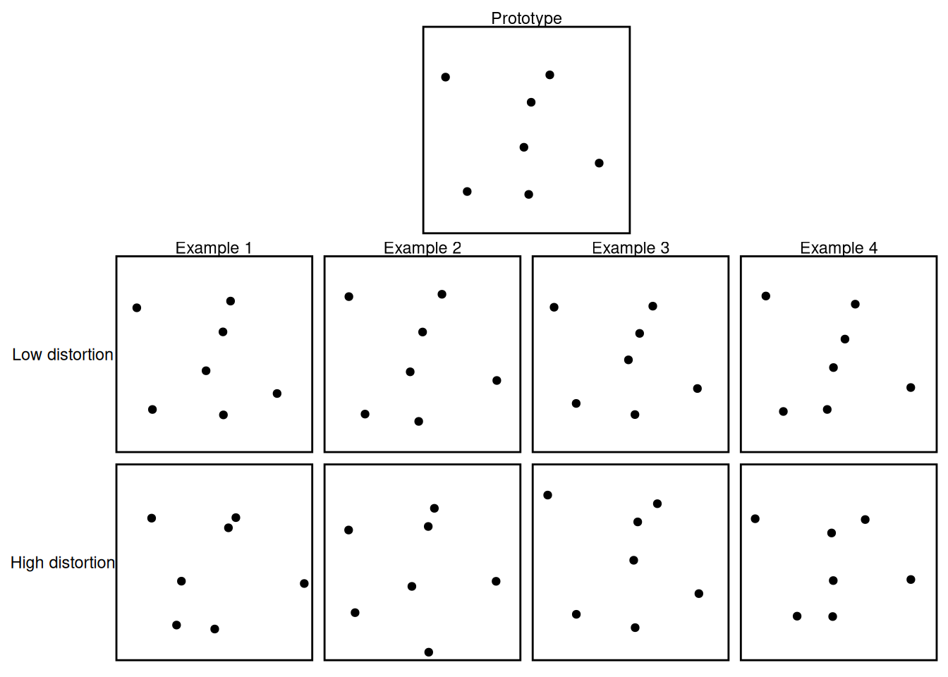
Each dot pattern was a distortion of a “prototype” dot pattern. As shown above, there could be “low distortions” which differ only a little from the prototype as well as “high distortions” which differ more strongly from the prototype. Collectively, the various distortions from a prototype share a “family resemblance” to one another. In that sense, they mimic the “dog” example from earlier, where even though all dogs look different, they can be understood as “variations on a theme”. The “theme” is a prototype, and we will now see that an autoencoder can learn a representation of the regularities that define such a prototype.
The example below uses a simplified version of the Posner & Keele (1968) paradigm. Each prototype is a sequence of binary symbols, which we might think of as indicating the presence or absence of different features. In the example below, there are two prototypes, perhaps representing two different diseases or two different concepts. The two prototypes differ on the first six features but match on the final two, perhaps like two different diseases with shared symptoms or two concepts with shared features.
On each epoch of training, the network is presented with a number of exemplars of each prototype. Each exemplar consists of a set of features, and there is a variable p_change that indicates the probability that any given feature of an exemplar will be “flipped” relative to its value in the prototype. For example, if the prototype is c(1, 1, 1, 0, 0, 0, 0, 1), then an exemplar is initially created that is an exact copy of that prototype. If p_change is greater than zero, then there is a chance that any one of the features of the exemplar could be flipped. For example, if the third feature is flipped, the resulting exemplar would be c(1, 1, 0, 0, 0, 0, 0, 1).
To begin, let’s see what happens if we only give the network 2 hidden units to work with. This is essentially forcing the model to “make do” with an internal representation of with only two dimensions. If the network is able to pick up on the patterns of family resemblance, then the activation of the two hidden units should reflect which of the two prototypes most likely generated any given exemplar. Below, p_change is set to 0.1. Let’s see how well the model does!
Code
logistic_act <- function(x) {
    return(1 / (1 + exp(-x)))
}

prototypes <- matrix(c(
    1, 1, 1, 0, 0, 0, 0, 1,
    0, 0, 0, 1, 1, 1, 0, 1
), nrow = 2, ncol = 8, byrow = TRUE,
dimnames = list(
    c("P1", "P2")
))

# On each epoch, the model sees a new randomly generated set of exemplars generated from each prototype
n_epochs <- 5000
# This is the number of exemplars of each prototype per epoch
n_per_prototype <- 100
# This is what proportion of features, on average, will differ between the exemplars and their prototype
p_change <- 0.1

learning_rate <- 0.1
n_hidden <- 2

i_to_h_assc_weights <- matrix(rnorm(n = ncol(prototypes) * n_hidden), nrow = ncol(prototypes), ncol = n_hidden) * 0.01
h_to_o_assc_weights <- matrix(rnorm(n = n_hidden * ncol(prototypes)), nrow = n_hidden, ncol = ncol(prototypes)) * 0.01

hidden_baseline <- rnorm(n = n_hidden) * 0.01
output_baseline <- rnorm(n = ncol(prototypes)) * 0.01

for (epoch in 1:n_epochs) {
    event <- prototypes[sample(rep(1:nrow(prototypes), each = n_per_prototype)), , drop = FALSE]
    to_change <- matrix(rbinom(n = nrow(event) * ncol(event), size = 1, p = p_change), nrow = nrow(event), ncol = ncol(event))
    event[to_change] <- 1 - event[to_change]

    target <- event

    d_h_to_o <- 0 * h_to_o_assc_weights
    d_i_to_h <- 0 * i_to_h_assc_weights

    d_h_baseline <- 0 * hidden_baseline
    d_o_baseline <- 0 * output_baseline

    prev_hidden_activation <- rep(0, n_hidden)

    for (i in 1:nrow(event)) {
        # Forward propagation (prediction)
        hidden_activation <- logistic_act(as.vector(event[i,] %*% i_to_h_assc_weights) + hidden_baseline)
        output_activation <- logistic_act(as.vector(hidden_activation %*% h_to_o_assc_weights) + output_baseline)

        # Compute error at output layer
        output_error <- target[i,] - output_activation

        # Back propagation (learning)

        # Derivative of error with respect to output unit activation
        d_output_error <- output_error * output_activation * (1 - output_activation)

        # Derivative of error with respect to hidden unit activation
        d_hidden_error <- as.vector(h_to_o_assc_weights %*% d_output_error) * hidden_activation * (1 - hidden_activation)

        # How much to adjust the associative weights between the hidden and output layers
        d_h_to_o <- d_h_to_o + learning_rate * outer(hidden_activation, d_output_error)

        # How much to adjust the associative weights between the input and hidden layers
        d_i_to_h <- d_i_to_h + learning_rate * outer(event[i,], d_hidden_error)

        # How much to adjust the baseline of the output units
        d_o_baseline <- learning_rate * d_output_error

        # How much to adjust the baseline of the hidden units
        d_h_baseline <- learning_rate * d_hidden_error
    }

    # Adjust weights
    i_to_h_assc_weights <- i_to_h_assc_weights + d_i_to_h
    h_to_o_assc_weights <- h_to_o_assc_weights + d_h_to_o

    hidden_baseline <- hidden_baseline + d_h_baseline
    output_baseline <- output_baseline + d_o_baseline
}

transfer_event <- diag(ncol(prototypes))
rownames(transfer_event) <- colnames(transfer_event) <- paste("Feature", 1:nrow(transfer_event))

transfer_hidden_activation <- matrix(0, nrow = nrow(transfer_event), ncol = n_hidden, dimnames = list(rownames(transfer_event), 1:n_hidden))
p_resp <- matrix(0, nrow = nrow(transfer_event), ncol = ncol(target), dimnames = list(rownames(transfer_event), colnames(target)))

for (i in 1:nrow(transfer_event)) {
    transfer_hidden_activation[i,] <- logistic_act(as.vector(transfer_event[i,] %*% i_to_h_assc_weights) + hidden_baseline)
    p_resp[i,] <- logistic_act(as.vector(transfer_hidden_activation[i,] %*% h_to_o_assc_weights) + output_baseline)
}
At the end of the chunk above, we probe what the model has learned by presenting it with eight “transfer” events each consisting of one of the eight features being set to 1 while the others are set to 0:
Code
knitr::kable(transfer_event)| Feature 1 | Feature 2 | Feature 3 | Feature 4 | Feature 5 | Feature 6 | Feature 7 | Feature 8 | |
|---|---|---|---|---|---|---|---|---|
| Feature 1 | 1 | 0 | 0 | 0 | 0 | 0 | 0 | 0 |
| Feature 2 | 0 | 1 | 0 | 0 | 0 | 0 | 0 | 0 |
| Feature 3 | 0 | 0 | 1 | 0 | 0 | 0 | 0 | 0 |
| Feature 4 | 0 | 0 | 0 | 1 | 0 | 0 | 0 | 0 |
| Feature 5 | 0 | 0 | 0 | 0 | 1 | 0 | 0 | 0 |
| Feature 6 | 0 | 0 | 0 | 0 | 0 | 1 | 0 | 0 |
| Feature 7 | 0 | 0 | 0 | 0 | 0 | 0 | 1 | 0 |
| Feature 8 | 0 | 0 | 0 | 0 | 0 | 0 | 0 | 1 |
The table below indicates the activation at the model’s “output” layer for each of the transfer events above, representing its expectations for the other feature values:
Code
knitr::kable(p_resp)| Feature 1 | 0.9997033 | 0.9893001 | 0.9893061 | 0.0106886 | 0.0107070 | 0.0106903 | 0.0018336 | 0.9981642 |
| Feature 2 | 0.9987015 | 0.9682807 | 0.9683123 | 0.0316595 | 0.0317569 | 0.0316688 | 0.0029465 | 0.9970532 |
| Feature 3 | 0.9987136 | 0.9685302 | 0.9685615 | 0.0314105 | 0.0315071 | 0.0314198 | 0.0029452 | 0.9970544 |
| Feature 4 | 0.0774881 | 0.0077560 | 0.0077707 | 0.9922162 | 0.9922614 | 0.9922206 | 0.0021182 | 0.9978799 |
| Feature 5 | 0.0765345 | 0.0077274 | 0.0077421 | 0.9922447 | 0.9922901 | 0.9922491 | 0.0021584 | 0.9978398 |
| Feature 6 | 0.0790053 | 0.0079269 | 0.0079419 | 0.9920447 | 0.9920909 | 0.9920491 | 0.0021339 | 0.9978642 |
| Feature 7 | 0.8709508 | 0.3250548 | 0.3254244 | 0.6742455 | 0.6753852 | 0.6743548 | 0.0034501 | 0.9965506 |
| Feature 8 | 0.9168317 | 0.3092547 | 0.3094502 | 0.6903754 | 0.6909781 | 0.6904331 | 0.0010764 | 0.9989210 |
We can see that the network has largely learned to expect feature values consistent with the prototype that is most closely associated with the activated feature. Of course, for the final two features which have the same value in both prototypes, the model’s expectations are more equivocal.
It is intriguing to note that, for the transfer pattern in which Feature 7 is “turned on”, the model still expects this feature to have a very low value! This feature had the value “0” in both prototypes, so the model would have only experienced a value of 1 for Feature 7 if it happened to be “flipped” by chance in one of the training examples. So in a sense, by expecting Feature 7 to have a value of 0 even when the model is “told” that it has a value of 1, the model is “discounting” the evidence of its “senses”!
By examining the patterns of hidden unit activation for each transfer pattern, we can see the source of the model’s expectations:
Code
knitr::kable(transfer_hidden_activation)| 1 | 2 | |
|---|---|---|
| Feature 1 | 0.9908998 | 0.1121541 |
| Feature 2 | 0.8531575 | 0.1670194 |
| Feature 3 | 0.8538664 | 0.1663734 |
| Feature 4 | 0.2083492 | 0.8811281 |
| Feature 5 | 0.2061844 | 0.8799589 |
| Feature 6 | 0.2094186 | 0.8787193 |
| Feature 7 | 0.4976117 | 0.4998254 |
| Feature 8 | 0.6069245 | 0.5975704 |
As we might have hoped, the model has learned to use its two hidden units to indicate which of the two prototypes is most consistent with the features in each transfer event. Once again, the final two (ambiguous) features also result in close-to-equal activation of each hidden unit.
That said, it might be more fair to judge the model if we don’t “give it the answer” by only equipping it with two hidden units. Let’s instead give it eight hidden units—the same number as there are features—and see if it can still discover the regularities consistent with each prototype.
Code
logistic_act <- function(x) {
    return(1 / (1 + exp(-x)))
}

prototypes <- matrix(c(
    1, 1, 1, 0, 0, 0, 0, 1,
    0, 0, 0, 1, 1, 1, 0, 1
), nrow = 2, ncol = 8, byrow = TRUE,
dimnames = list(
    c("P1", "P2")
))

# On each epoch, the model sees a new randomly generated set of exemplars generated from each prototype
n_epochs <- 5000
# This is the number of exemplars of each prototype per epoch
n_per_prototype <- 100
# This is what proportion of features, on average, will differ between the exemplars and their prototype
p_change <- 0.1

learning_rate <- 0.1
n_hidden <- 8

i_to_h_assc_weights <- matrix(rnorm(n = ncol(prototypes) * n_hidden), nrow = ncol(prototypes), ncol = n_hidden) * 0.01
h_to_o_assc_weights <- matrix(rnorm(n = n_hidden * ncol(prototypes)), nrow = n_hidden, ncol = ncol(prototypes)) * 0.01

hidden_baseline <- rnorm(n = n_hidden) * 0.01
output_baseline <- rnorm(n = ncol(prototypes)) * 0.01

for (epoch in 1:n_epochs) {
    event <- prototypes[sample(rep(1:nrow(prototypes), each = n_per_prototype)), , drop = FALSE]
    to_change <- matrix(rbinom(n = nrow(event) * ncol(event), size = 1, p = p_change), nrow = nrow(event), ncol = ncol(event))
    event[to_change] <- 1 - event[to_change]

    target <- event

    d_h_to_o <- 0 * h_to_o_assc_weights
    d_i_to_h <- 0 * i_to_h_assc_weights

    d_h_baseline <- 0 * hidden_baseline
    d_o_baseline <- 0 * output_baseline

    prev_hidden_activation <- rep(0, n_hidden)

    for (i in 1:nrow(event)) {
        # Forward propagation (prediction)
        hidden_activation <- logistic_act(as.vector(event[i,] %*% i_to_h_assc_weights) + hidden_baseline)
        output_activation <- logistic_act(as.vector(hidden_activation %*% h_to_o_assc_weights) + output_baseline)

        # Compute error at output layer
        output_error <- target[i,] - output_activation

        # Back propagation (learning)

        # Derivative of error with respect to output unit activation
        d_output_error <- output_error * output_activation * (1 - output_activation)

        # Derivative of error with respect to hidden unit activation
        d_hidden_error <- as.vector(h_to_o_assc_weights %*% d_output_error) * hidden_activation * (1 - hidden_activation)

        # How much to adjust the associative weights between the hidden and output layers
        d_h_to_o <- d_h_to_o + learning_rate * outer(hidden_activation, d_output_error)

        # How much to adjust the associative weights between the input and hidden layers
        d_i_to_h <- d_i_to_h + learning_rate * outer(event[i,], d_hidden_error)

        # How much to adjust the baseline of the output units
        d_o_baseline <- learning_rate * d_output_error

        # How much to adjust the baseline of the hidden units
        d_h_baseline <- learning_rate * d_hidden_error
    }

    # Adjust weights
    i_to_h_assc_weights <- i_to_h_assc_weights + d_i_to_h
    h_to_o_assc_weights <- h_to_o_assc_weights + d_h_to_o

    hidden_baseline <- hidden_baseline + d_h_baseline
    output_baseline <- output_baseline + d_o_baseline
}

transfer_event <- diag(ncol(prototypes))
rownames(transfer_event) <- colnames(transfer_event) <- paste("Feature", 1:nrow(transfer_event))

transfer_hidden_activation <- matrix(0, nrow = nrow(transfer_event), ncol = n_hidden, dimnames = list(rownames(transfer_event), 1:n_hidden))
p_resp <- matrix(0, nrow = nrow(transfer_event), ncol = ncol(target), dimnames = list(rownames(transfer_event), colnames(target)))

for (i in 1:nrow(transfer_event)) {
    transfer_hidden_activation[i,] <- logistic_act(as.vector(transfer_event[i,] %*% i_to_h_assc_weights) + hidden_baseline)
    p_resp[i,] <- logistic_act(as.vector(transfer_hidden_activation[i,] %*% h_to_o_assc_weights) + output_baseline)
}
Code
knitr::kable(p_resp)| Feature 1 | 0.9999629 | 0.9873418 | 0.9873510 | 0.0126542 | 0.0126575 | 0.0126505 | 0.0008719 | 0.9991304 |
| Feature 2 | 0.9993704 | 0.9234755 | 0.9237602 | 0.0763888 | 0.0764785 | 0.0763762 | 0.0018163 | 0.9981896 |
| Feature 3 | 0.9993676 | 0.9230696 | 0.9233528 | 0.0768033 | 0.0768983 | 0.0768017 | 0.0018001 | 0.9982057 |
| Feature 4 | 0.1704360 | 0.0068217 | 0.0068725 | 0.9931383 | 0.9931712 | 0.9931460 | 0.0010124 | 0.9989944 |
| Feature 5 | 0.1709796 | 0.0068199 | 0.0068703 | 0.9931409 | 0.9931733 | 0.9931486 | 0.0010069 | 0.9989999 |
| Feature 6 | 0.1688919 | 0.0067943 | 0.0068453 | 0.9931664 | 0.9931986 | 0.9931735 | 0.0010205 | 0.9989865 |
| Feature 7 | 0.9243916 | 0.1953597 | 0.1963633 | 0.8039330 | 0.8044775 | 0.8040272 | 0.0017631 | 0.9982449 |
| Feature 8 | 0.9688339 | 0.2665740 | 0.2675084 | 0.7328589 | 0.7333190 | 0.7329245 | 0.0009362 | 0.9990692 |
Even without encouraging the model to find the “right” answer, it still looks like it is able to form reasonable expectations for the feature values that are consistent with the prototypes that originally generated the training exemplars.
However, since there are now 8 hidden units, its a bit hard to see how the pattern of activation among the hidden units represents each potential prototype:
Code
knitr::kable(transfer_hidden_activation)| 1 | 2 | 3 | 4 | 5 | 6 | 7 | 8 | |
|---|---|---|---|---|---|---|---|---|
| Feature 1 | 0.1528907 | 0.4344921 | 0.1661314 | 0.1710326 | 0.9538300 | 0.9649348 | 0.9494558 | 0.1816092 |
| Feature 2 | 0.2329792 | 0.4075160 | 0.2372756 | 0.2541759 | 0.7525858 | 0.7815335 | 0.7455288 | 0.2541011 |
| Feature 3 | 0.2375500 | 0.4140858 | 0.2341705 | 0.2548858 | 0.7512986 | 0.7846717 | 0.7425981 | 0.2524576 |
| Feature 4 | 0.7721480 | 0.6340845 | 0.7706312 | 0.7539505 | 0.3059169 | 0.2862130 | 0.3127077 | 0.7517998 |
| Feature 5 | 0.7744988 | 0.6328773 | 0.7695565 | 0.7554082 | 0.3045691 | 0.2868571 | 0.3155504 | 0.7514157 |
| Feature 6 | 0.7715945 | 0.6332336 | 0.7680214 | 0.7554003 | 0.3055191 | 0.2870289 | 0.3088729 | 0.7534171 |
| Feature 7 | 0.4976473 | 0.5002462 | 0.5005177 | 0.5032810 | 0.4940626 | 0.4956329 | 0.4955740 | 0.4910196 |
| Feature 8 | 0.5082826 | 0.5433736 | 0.5123282 | 0.5144572 | 0.5748479 | 0.5941206 | 0.5741431 | 0.5155124 |
So let’s make a plot instead:
Code
array2DF(transfer_hidden_activation) %>%
    mutate(transfer_event = factor(Var1)) %>%
    mutate(hidden_unit_index = as.numeric(Var2)) %>%
    ggplot(aes(x = hidden_unit_index, y = Value, color = transfer_event)) +
    geom_line() +
    scale_color_okabeito() +
    labs(x = "Hidden unit index", y = "Activation", color = "Active feature")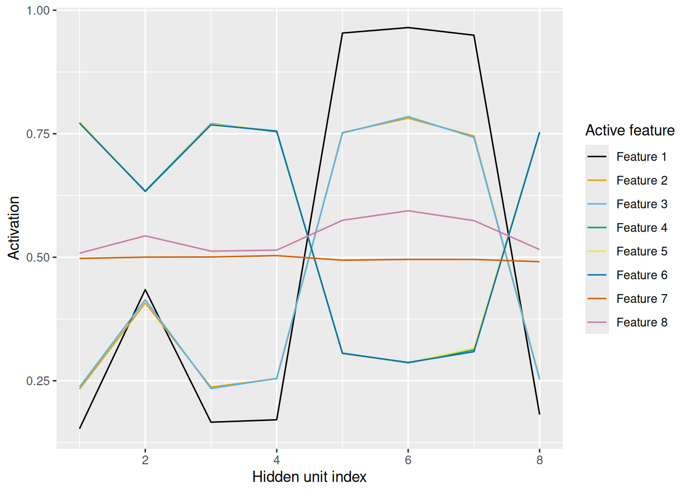
The visualization makes it easier to see that the pattern of hidden unit activation is essentially “mirrored” between features 1–3 and features 4–6, and flat for the ambiguous features 7 and 8. Once again, the network has learned to form a distributed representation of its input that captures the regularities of the events that it has experienced.
12.4 Simple recurrent networks: Learning patterns in time
One of the most interesting (in my opinion) applications of backprop networks comes in the form of simple recurrent networks (SRN). These were described by Elman (1990), who showed that they could learn structure in time. These models are applied to sequences, where the current event in the sequence is treated as “input” and the next event is the target at the output layer. Thus, these networks are explicitly trained to predict the future.
In principle, the same model structure we’ve seen so far could work here too. But Elman (1990) proposed an interesting change: The input on each step of the sequence isn’t just the current event—it is also the vector of hidden unit activation from the previous step of the sequence. Thus, the networks own prior state is treated as input for the purpose of making a prediction. This means that the hidden unit representations learned by the network must pull “double duty”—they need to learn, in essence, how to serve as useful memory representations.
12.4.1 Learning to have memory
Elman (1990) gave a simple illustration of an SRN learning to have memory. In the following example, each event has just a single dimension—it can be 0 or 1. Sequences are comprised of three-element subsequences. Within each subsequence, the final element is the “exclusive-or” (XOR) of the previous two elements. Specifically, the final element is 1 if the previous two elements are different and it is 0 if the previous two elements are the same. These three-element subsequences are randomly concatenated to form a long exposure sequence.
This is a challenging pattern to learn! In many cases, it will be impossible to predict the next element. Imagine that the sequence 0, 1, 1 occurs. When the first element occurs, it is not possible to predict what the second one will be. However, once the second element occurs, it is possible to predict the third element, since it follows the XOR rule. But once the third element occurs, it is again impossible to predict the next element, since the next element is the start of the next sequence. Only for the second element of a sequence is it possible to make a reasonable prediction about the next element. And that’s only if you (a) can remember far enough back; and (b) have learned the XOR rule.
This learning situation can be thought of as a microcosm for learning the structure of events more generally. For example, if a pitcher throws a ball, we cannot predict whether the batter will hit it. But once we know whether the batter has hit the ball or not, we can form some expectation about what will happen next. But then the next pitch is unpredictable once again.
The code below implements a version of Elman’s XOR sequence task. The network only has 2 hidden units. It learns in batches, where each batch is a long sequence built by concatenating many 3-element subsequences, each of which follow the XOR rule.
Code
logistic_act <- function(x) {
    return(1 / (1 + exp(-x)))
}

# Each row is a subsequence from which the whole training sequence will be built.
# The number refer to the rows in the "representations" matrix below.
subsequences <- matrix(c(
    1, 1, 2,
    1, 2, 1,
    2, 1, 1,
    2, 2, 2
), nrow = 4, ncol = 3, byrow = TRUE)

representations <- matrix(c(
    1,
    0
), nrow = 2, ncol = 1, byrow = TRUE)

# On each epoch, the model learns on a new randomly generated training sequence
n_epochs <- 5000
# This is the number of times each subsequence will occur in each training sequence
n_per_subsequence <- 100

learning_rate <- 0.1
n_hidden <- 2

i_to_h_assc_weights <- matrix(rnorm(n = (ncol(representations) + n_hidden) * n_hidden), nrow = ncol(representations) + n_hidden, ncol = n_hidden) * 0.01
h_to_o_assc_weights <- matrix(rnorm(n = n_hidden * ncol(representations)), nrow = n_hidden, ncol = ncol(representations)) * 0.01

hidden_baseline <- rnorm(n = n_hidden) * 0.01
output_baseline <- rnorm(n = ncol(representations)) * 0.01

for (epoch in 1:n_epochs) {
    training_sequence <- c(t(subsequences[sample(rep(1:nrow(subsequences), each = n_per_subsequence)),]))

    event <- representations[training_sequence[1:(length(training_sequence) - 1)], , drop = FALSE]

    target <- representations[training_sequence[2:length(training_sequence)], , drop = FALSE]

    d_h_to_o <- 0 * h_to_o_assc_weights
    d_i_to_h <- 0 * i_to_h_assc_weights

    d_h_baseline <- 0 * hidden_baseline
    d_o_baseline <- 0 * output_baseline

    prev_hidden_activation <- rep(0, n_hidden)

    for (i in 1:nrow(event)) {
        # Forward propagation (prediction)
        this_input <- c(event[i,], prev_hidden_activation)
        hidden_activation <- logistic_act(as.vector(this_input %*% i_to_h_assc_weights) + hidden_baseline)
        output_activation <- logistic_act(as.vector(hidden_activation %*% h_to_o_assc_weights) + output_baseline)

        # Compute error at output layer
        output_error <- target[i,] - output_activation

        # Back propagation (learning)

        # Derivative of error with respect to output unit activation
        d_output_error <- output_error * output_activation * (1 - output_activation)

        # Derivative of error with respect to hidden unit activation
        d_hidden_error <- as.vector(h_to_o_assc_weights %*% d_output_error) * hidden_activation * (1 - hidden_activation)

        # How much to adjust the associative weights between the hidden and output layers
        d_h_to_o <- d_h_to_o + learning_rate * outer(hidden_activation, d_output_error)

        # How much to adjust the associative weights between the input and hidden layers
        d_i_to_h <- d_i_to_h + learning_rate * outer(this_input, d_hidden_error)

        # How much to adjust the baseline of the output units
        d_o_baseline <- learning_rate * d_output_error

        # How much to adjust the baseline of the hidden units
        d_h_baseline <- learning_rate * d_hidden_error

        # Copy hidden unit activation
        prev_hidden_activation <- hidden_activation
    }

    # Adjust weights
    i_to_h_assc_weights <- i_to_h_assc_weights + d_i_to_h
    h_to_o_assc_weights <- h_to_o_assc_weights + d_h_to_o

    hidden_baseline <- hidden_baseline + d_h_baseline
    output_baseline <- output_baseline + d_o_baseline
}

transfer_sequence <- c(t(subsequences[sample(rep(1:nrow(subsequences), each = n_per_subsequence)),]))

event <- representations[transfer_sequence[1:(length(transfer_sequence) - 1)], , drop = FALSE]

target <- representations[transfer_sequence[2:length(transfer_sequence)], , drop = FALSE]

transfer_error <- rep(0, nrow(event))

prev_hidden_activation <- rep(0, n_hidden)

for (i in 1:nrow(event)) {
    this_input <- c(event[i,], prev_hidden_activation)
    hidden_activation <- logistic_act(as.vector(this_input %*% i_to_h_assc_weights) + hidden_baseline)
    output_activation <- logistic_act(as.vector(hidden_activation %*% h_to_o_assc_weights) + output_baseline)
    transfer_error[i] <- sqrt(mean((target[i,] - output_activation)^2))
    prev_hidden_activation <- hidden_activation
}

tibble(step = 1:nrow(event), error = transfer_error) %>%
    mutate(sub_step = ((step - 1) %% ncol(subsequences)) + 1) %>%
    ggplot(aes(x = sub_step, y = error)) +
    stat_summary(fun = mean, geom = "line", group = 1) +
    stat_summary(fun.data = mean_cl_normal) +
    labs(x = "Position within subsequence", y = "Root mean squared prediction error")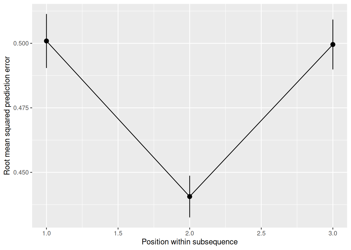
As we can see, once trained, the network shows exactly the “dip” in prediction error that we would expect if the network (a) could use its hidden layer to retain memory sufficient for the task; and (b) had learned the XOR pattern.
12.4.2 Learning concept representations by prediction
The following illustrates how the same SRN model structure can learn to distinguish between more complex concepts based on how they occur within “sentences” of a “language”. Specifically, the network will be presented with a sequence consisting of concatenated subsequences, each of which is three elements long. These elements comprise “sentences” following a “subject-verb-object” frame. Only some items can serve as each category, some subjects can engage in different verbs, and some objects can only receive certain verbs.
Code
logistic_act <- function(x) {
    return(1 / (1 + exp(-x)))
}

# Each row is a subsequence from which the whole training sequence will
# be built.
subsequences <- matrix(c(
    1, 5, 2,
    1, 5, 3,
    1, 5, 4,
    1, 6, 2,
    1, 6, 3,
    1, 7, 3,
    1, 8, 4,
    2, 5, 1,
    2, 5, 3,
    2, 5, 4,
    2, 6, 1,
    2, 6, 3,
    2, 7, 3,
    2, 8, 3, # (only the dog can throw the door)
    2, 8, 4
), nrow = 15, ncol = 3, byrow = TRUE)

representations <- diag(8)
rownames(representations) <- colnames(representations) <- c("cat", "dog", "door", "rock", "see", "hear", "use", "throw")

# On each epoch, the model learns on a new randomly generated training sequence
n_epochs <- 10000
# This is the number of times each subsequence will occur in each training sequence
n_per_subsequence <- 10

learning_rate <- 0.1
n_hidden <- 7

n_hidden_snapshots <- 9
epoch_to_snap <- round(exp(seq(0, log(n_epochs), length.out = n_hidden_snapshots)))
snapshot_hidden_activation <- array(0, dim = c(n_hidden_snapshots, nrow(representations), n_hidden), dimnames = list("epoch" = epoch_to_snap, "item" = rownames(representations), "hidden_unit" = 1:n_hidden))

i_to_h_assc_weights <- matrix(rnorm(n = (ncol(representations) + n_hidden) * n_hidden), nrow = ncol(representations) + n_hidden, ncol = n_hidden) * 0.01
h_to_o_assc_weights <- matrix(rnorm(n = n_hidden * ncol(representations)), nrow = n_hidden, ncol = ncol(representations)) * 0.01

hidden_baseline <- rnorm(n = n_hidden) * 0.01
output_baseline <- rnorm(n = ncol(representations)) * 0.01

for (epoch in 1:n_epochs) {
    training_sequence <- c(t(subsequences[sample(rep(1:nrow(subsequences), each = n_per_subsequence)),]))

    event <- representations[training_sequence[1:(length(training_sequence) - 1)], , drop = FALSE]

    target <- representations[training_sequence[2:length(training_sequence)], , drop = FALSE]

    d_h_to_o <- 0 * h_to_o_assc_weights
    d_i_to_h <- 0 * i_to_h_assc_weights

    d_h_baseline <- 0 * hidden_baseline
    d_o_baseline <- 0 * output_baseline

    prev_hidden_activation <- rep(0, n_hidden)

    for (i in 1:nrow(event)) {
        # Forward propagation (prediction)
        this_input <- c(event[i,], prev_hidden_activation)
        hidden_activation <- logistic_act(as.vector(this_input %*% i_to_h_assc_weights) + hidden_baseline)
        output_activation <- logistic_act(as.vector(hidden_activation %*% h_to_o_assc_weights) + output_baseline)

        # Compute error at output layer
        output_error <- target[i,] - output_activation

        # Back propagation (learning)

        # Derivative of error with respect to output unit activation
        d_output_error <- output_error * output_activation * (1 - output_activation)

        # Derivative of error with respect to hidden unit activation
        d_hidden_error <- as.vector(h_to_o_assc_weights %*% d_output_error) * hidden_activation * (1 - hidden_activation)

        # How much to adjust the associative weights between the hidden and output layers
        d_h_to_o <- d_h_to_o + learning_rate * outer(hidden_activation, d_output_error)

        # How much to adjust the associative weights between the input and hidden layers
        d_i_to_h <- d_i_to_h + learning_rate * outer(this_input, d_hidden_error)

        # How much to adjust the baseline of the output units
        d_o_baseline <- learning_rate * d_output_error

        # How much to adjust the baseline of the hidden units
        d_h_baseline <- learning_rate * d_hidden_error

        # Copy hidden unit activation
        prev_hidden_activation <- hidden_activation
    }

    # Adjust weights
    i_to_h_assc_weights <- i_to_h_assc_weights + d_i_to_h
    h_to_o_assc_weights <- h_to_o_assc_weights + d_h_to_o

    hidden_baseline <- hidden_baseline + d_h_baseline
    output_baseline <- output_baseline + d_o_baseline

    if (epoch %in% as.numeric(dimnames(snapshot_hidden_activation)[[1]])) {
        prev_hidden_activation <- rep(0, n_hidden)

        for (i in 1:nrow(representations)) {
            snapshot_hidden_activation[as.character(epoch), i, ] <- logistic_act(as.vector(c(representations[i,], prev_hidden_activation) %*% i_to_h_assc_weights) + hidden_baseline)
        }
    }
}

array2DF(snapshot_hidden_activation) %>%
    mutate(item = factor(item, levels = rownames(representations))) %>%
    mutate(hidden_unit = as.numeric(hidden_unit)) %>%
    mutate(epoch = factor(epoch, levels = as.character(sort(unique(as.numeric(epoch)))))) %>%
    ggplot(aes(x = hidden_unit, y = Value, color = item)) +
    geom_line() +
    scale_color_brewer(palette = "Paired") +
    facet_wrap("epoch", labeller = label_both)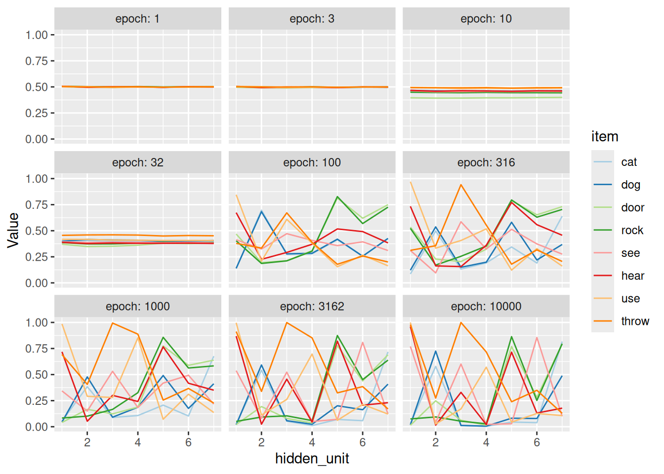
Code
item_mds <- array(0, dim = c(n_hidden_snapshots, nrow(representations), 2), dimnames = list("epoch" = epoch_to_snap, "item" = rownames(representations), "dim" = paste0("dim", 1:2)))

for (epoch in dimnames(snapshot_hidden_activation)[[1]]) {
    item_mds[epoch, , ] <- cmdscale(d = dist(snapshot_hidden_activation[epoch,,]), k = 2)
}

array2DF(item_mds) %>%
    pivot_wider(id_cols = c(epoch, item), names_from = dim, values_from = Value) %>%
    mutate(item = factor(item, levels = rownames(representations))) %>%
    mutate(epoch = factor(epoch, levels = as.character(sort(unique(as.numeric(epoch)))))) %>%
    ggplot(aes(x = dim1, y = dim2, color = item)) +
    geom_path() +
    coord_equal() +
    scale_color_brewer(palette = "Paired") +
    labs(title = "Evolution of internal representations with learning", x = "Dimension 1", y = "Dimension 2", caption = "Visualization by multidimensional scaling")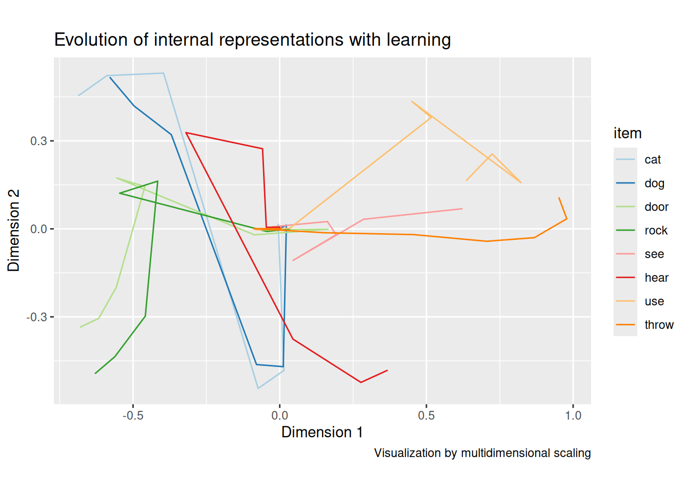
As we can see, the model learns to distinguish between nouns and verbs fairly quickly. Same goes for subjects (cat, dog) and objects (door, rock). Eventually, the individual items get differentiated, like we saw with the concepts at the beginning of the chapter. The key difference is that the SRN has learned these concept representations by virtue of how they enable it to predict the next items in the sequence, not in terms of clearly labeled features.
12.5 Exercises
- Adapt the concept-feature learning model so that it operates “in reverse”. In other words, swap the
targetandeventmatrices. The resulting model will thus learn to assign a concept name (oak, pine, etc.) to a set of features. Leaving everything else the same, run the model and comment on the nature of the representations it learns within its hidden units and compare them to the representations learned by the model in the chapter. - Try running the prototype-learning autoencoder model with different values of the
p_changevariable, leavingn_hiddenset to 8. See if you can find a value ofp_changeat which the model no longer shows any evidence of learning the two prototypes. Comment on what sorts of representations the model has learned, if indeed it has learned any structure at all! - Devise a learning situation that is relevant to your research and adapt one of the models from this chapter to apply it to that scenario. You will need to think about how you want to represent the features of each learning event and what the “target” is for the learner (e.g., are they learning to categorize events or choose an action, are they an “autoencoder”, are they learning to predict like an SRN?). You will also need to explore different values for the number of hidden units in the model, the learning rate, as well as the number of epochs and the number of learning events per epoch. In the end, describe the learning situation you devised and the settings required for your model to succeed in your learning task. Describe the nature of the hidden-layer representations the model seems to have learned as well as the trajectory (over epochs) by which the model appears to have learned those trajectories (e.g., did some distinctions get learned earlier than others?).