Lab 7 The normal distribution
The venerable normal distribution or “bell curve” is almost like a mascot for statistics. Although there are variables in real life that are distributed according to a normal distribution, its real value is in describing sampling distributions. We have seen sampling distributions in both hypothesis testing and confidence intervals: Sampling distributions represent the variability in a point estimate like a proportion or mean that is due to the randomness involved in selecting samples from a population. According to the central limit theorem, much of the time, sampling distributions will be approximately normal in shape.
In this session, we will first use the normal distribution as a model for population distributions, that is the distribution of values on a particular variable across a whole population. Along the way, we will get the hang of using R to find proportions and intervals based on the normal distribution. Then, in the second part, we will use the normal distribution as a model for sampling distributions. This will give us some insight into how standard error relates to things like sample size.
To help with the later exercises in this session, be sure to download the worksheet for this session by right-clicking on the following link and selecting “Save link as…”: Worksheet for Lab 7. Open the saved file (which by default is called “ws_lab07.Rmd”) in RStudio.
7.1 The data: National Health and Nutrition Examination Surveys (NHANES)
The data we will be using in this lab—labeled nhanes in your R environment—were originally collected by the US National Center for Heath Statistics between 2009 and 2012. This is a subset of what is effectively a simple random sample from the entire US population, though we will only use some of the observations out of the many they collected.
7.2 The normal distribution as a model for a population distribution
The variable we will focus on first is the number of hours people report sleeping each night, measured in hours. This is recorded for each individual in the sample under the variable SleepHrsNight.
7.2.1 Visualize the distribution
As usual, we begin by visualizing the actual data. As a reminder, we will assume for the time being that these data constitute the entire population of interest. The histogram below shows the population distribution of nightly hours of sleep:
nhanes %>%
    ggplot(aes(x = SleepHrsNight)) +
    geom_histogram(binwidth = 1)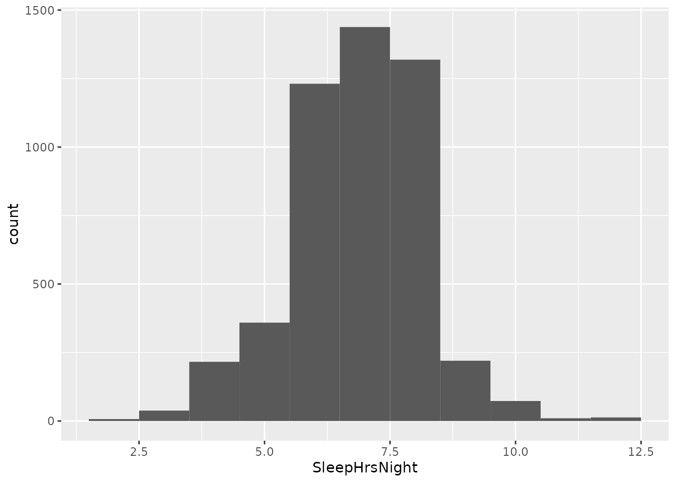
7.2.2 Is the normal distribution a good model?
Next, we want to know whether the normal distribution will be a good model of the population distribution we just visualized. To do this, we will draw a curve representing the normal distribution on top of the histogram we just made.
But remember that the normal distribution is just a shape. Its center and spread are determined by two population parameters: the mean (\(\mu\)) and standard deviation (\(\sigma\)). What should those parameters be?
Let’s first take a wild guess and say they should be \(\mu = 8\) and \(\sigma = 1\). We can draw this distribution using the chunk of code below:
nhanes %>%
    ggplot(aes(x = SleepHrsNight)) +
    geom_histogram(aes(y = ..density..), binwidth = 1) +
    stat_function(fun = dnorm, args = list(mean = 8, sd = 1), color = 'darkred')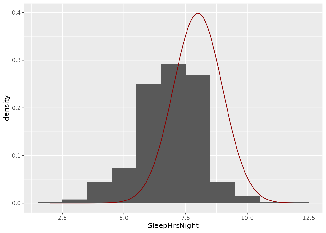
Notice that we needed to add aes(y = ..density..) to our histogram line, for reasons which will be clear in the next paragraph. The final line lets us draw a function on our graph. The function is called dnorm for “density of a normal distribution”. We had to say what the arguments of that function should be, which are a list in which we say what the mean and sd of the normal distribution should be.
The whole “density” thing comes from this: A histogram shows absolute counts. But a normal distribution only specifies the relative frequency of different values. The relative frequency is called the “density”. This is what the dnorm function gives us for the normal distribution. So adding aes(y = ..density..) to the histogram line told R to show the density (relative frequency) rather than the absolute counts.
Anyway, it is clear that a mean of 8 hours and standard deviation of 1 hour do not make a good fit.
Exercise 7.1 Play around with different values of “mean” and “sd” in the chunk of code below. Try to find values that result in a normal distribution that is a good “fit” to the data. You can start by setting mean = 8 and sd = 1 and then adjust from there.
nhanes %>%
    ggplot(aes(x = SleepHrsNight)) +
    geom_histogram(aes(y = ..density..), binwidth = 1) +
stat_function(fun = dnorm, args = list(mean = ___, sd = ___), color = 'darkred')- Describe the strategy you used to find values for
meanandsdthat seemed to make a good fit. - What values did you find?
- Try setting
mean = 6.86andsd = 1.32and run the chunk. These are close to the actual mean and standard deviation of the data in our sample. Compared to the settings formeanandsdthat you found, do you think these make a better or worse “fit”?
7.2.3 Bad days, bad models?
As part of the same survey, people were asked how many days out of the last 30 would they consider their mental health to have been poor. This is recorded under the variable named DaysMentHlthBad.
Exercise 7.2 Use the chunk of code to help you make a histogram of the distribution of bad mental health days per month (remember that these are recorded in the nhanes dataset under the variable named DaysMentHlthBad; you can also try different bin widths as you like).
___ %>%
    ggplot(aes(x = ___)) +
geom_histogram(binwidth = 1)- Do you think the normal distribution would be able to fit these data? Why or why not?
- Make a reasonable guess about why the population distribution might have the shape that it has, taking note of the fact that respondents had to give a number of days out of 30.
7.3 The normal distribution as a model for a sampling distribution
In the previous section, we got a sense of how we can sometimes use the normal distribution to approximate a distribution of observed values from a population. But more often, the normal distribution is used as a model of a sampling distribution.
In this section, we will again assume that the nhanes dataset represents the entire population of interest. We will simulate drawing many different samples of different sizes from this population and calculate a summary statistic on each sample. The sampling distribution is the distribution of those summary statistics and we will see how well we can approximate it with a normal distribution.
We will focus on just one of the questions asked on the NHANES survey. This question asks whether someone has ever tried using marijuana. This information resides in the variable Marijuana and a person’s response is either “Yes” or “No”.
Exercise 7.3 Without even looking at the data, would it make sense to try to use a normal distribution to approximate the population distribution of the responses to the Marijuana question? Why or why not?
7.3.1 The “true” proportion
Because we are assuming that the nhanes data represent the entire population we are interested in, we can find the “true” value of the population parameter \(\pi_{\text{Marijuana}}\), that is, the proportion of people who have ever tried marijuana. We can use the code below:
nhanes %>%
    specify(response = Marijuana, success = "Yes") %>%
    calculate(stat = "prop")
## Response: Marijuana (factor)
## # A tibble: 1 × 1
## stat
## <dbl>
## 1 0.5857.3.2 Simulating many samples
Last session, we used bootstrapping to simulate what would happen if we collected many samples from a population. We did that by using our sample to estimate the whole population. Now, we have access to that whole population. We can therefore draw as many samples of a given size as we want!
The following chunk of code randomly samples 5 people from the population and gets R to remember that sample under the name sample_size5.
sample_size5 <- nhanes %>%
    slice_sample(n = 5)
This is what that sample looks like:
| ID | SurveyYr | Gender | Age | AgeDecade | AgeMonths | Race1 | Race3 | Education | MaritalStatus | HHIncome | HHIncomeMid | Poverty | HomeRooms | HomeOwn | Work | Weight | Length | HeadCirc | Height | BMI | BMICatUnder20yrs | BMI_WHO | Pulse | BPSysAve | BPDiaAve | BPSys1 | BPDia1 | BPSys2 | BPDia2 | BPSys3 | BPDia3 | Testosterone | DirectChol | TotChol | UrineVol1 | UrineFlow1 | UrineVol2 | UrineFlow2 | Diabetes | DiabetesAge | HealthGen | DaysPhysHlthBad | DaysMentHlthBad | LittleInterest | Depressed | nPregnancies | nBabies | Age1stBaby | SleepHrsNight | SleepTrouble | PhysActive | PhysActiveDays | TVHrsDay | CompHrsDay | TVHrsDayChild | CompHrsDayChild | Alcohol12PlusYr | AlcoholDay | AlcoholYear | SmokeNow | Smoke100 | Smoke100n | SmokeAge | Marijuana | AgeFirstMarij | RegularMarij | AgeRegMarij | HardDrugs | SexEver | SexAge | SexNumPartnLife | SexNumPartYear | SameSex | SexOrientation | PregnantNow |
|---|---|---|---|---|---|---|---|---|---|---|---|---|---|---|---|---|---|---|---|---|---|---|---|---|---|---|---|---|---|---|---|---|---|---|---|---|---|---|---|---|---|---|---|---|---|---|---|---|---|---|---|---|---|---|---|---|---|---|---|---|---|---|---|---|---|---|---|---|---|---|---|---|---|---|---|
| 65978 | 2011_12 | male | 57 | 50-59 | NA | White | White | Some College | NeverMarried | 25000-34999 | 30000 | 2.86 | 5 | Own | Working | 104.5 | NA | NA | 174.4 | 34.40 | NA | 30.0_plus | 66 | 141 | 79 | 122 | 78 | 134 | 78 | 148 | 80 | 545.84 | 0.83 | 5.61 | 69 | 0.473 | NA | NA | No | NA | Good | 5 | 0 | None | None | NA | NA | NA | 8 | No | No | NA | 1_hr | 1_hr | NA | NA | Yes | 4 | 24 | Yes | Yes | Smoker | 23 | Yes | 23 | No | NA | No | Yes | 23 | 4 | 1 | No | Heterosexual | NA |
| 53457 | 2009_10 | female | 30 | 30-39 | 364 | Mexican | NA | 8th Grade | Married | NA | NA | NA | 5 | Own | NotWorking | 64.7 | NA | NA | 159.5 | 25.43 | NA | 25.0_to_29.9 | 72 | 104 | 58 | 104 | 58 | 104 | 56 | 104 | 60 | NA | 1.47 | 5.90 | 212 | 1.076 | NA | NA | No | NA | Vgood | 0 | 0 | None | None | 2 | 1 | NA | 9 | No | No | NA | NA | NA | NA | NA | No | NA | NA | NA | No | Non-Smoker | NA | No | NA | No | NA | No | Yes | 23 | 1 | 0 | No | Heterosexual | Unknown |
| 53965 | 2009_10 | male | 31 | 30-39 | 375 | Mexican | NA | Some College | Married | 65000-74999 | 70000 | 4.94 | 5 | Rent | NotWorking | 95.0 | NA | NA | 175.7 | 30.77 | NA | 30.0_plus | 66 | 108 | 75 | 114 | 74 | 110 | 74 | 106 | 76 | NA | 1.40 | 5.72 | 84 | 0.124 | NA | NA | No | NA | Good | 14 | 0 | None | None | NA | NA | NA | 7 | No | Yes | 3 | NA | NA | NA | NA | Yes | 1 | 48 | NA | No | Non-Smoker | NA | Yes | 16 | No | NA | No | Yes | 18 | 5 | 1 | No | Heterosexual | NA |
| 54006 | 2009_10 | male | 20 | 20-29 | 240 | Mexican | NA | Some College | NeverMarried | 75000-99999 | 87500 | 2.54 | 5 | Own | Working | 60.0 | NA | NA | 170.1 | 20.74 | NA | 18.5_to_24.9 | 62 | 105 | 62 | 108 | 62 | 108 | 64 | 102 | 60 | NA | 0.96 | 4.45 | 145 | NA | NA | NA | No | NA | Good | 0 | 1 | None | None | NA | NA | NA | 10 | No | Yes | 3 | NA | NA | NA | NA | No | NA | NA | NA | No | Non-Smoker | NA | Yes | 15 | No | NA | No | Yes | 16 | 1 | 1 | No | Heterosexual | NA |
| 63200 | 2011_12 | female | 59 | 50-59 | NA | White | White | College Grad | Married | more 99999 | 100000 | 5.00 | 7 | Own | Working | 65.1 | NA | NA | 155.6 | 26.90 | NA | 25.0_to_29.9 | 70 | 139 | 73 | 142 | 66 | 142 | 74 | 136 | 72 | 4.37 | 1.89 | 5.90 | 179 | 1.432 | NA | NA | No | NA | Good | 0 | 20 | None | None | 2 | 1 | NA | 8 | No | Yes | 6 | 4_hr | 0_to_1_hr | NA | NA | Yes | 2 | 364 | No | Yes | Smoker | 18 | Yes | 18 | No | NA | No | Yes | 19 | 3 | 1 | No | Heterosexual | NA |
Notice that we still have all of those people’s responses to each question on the NHANES survey. That means we can get a summary statistic for the Marijuana variable from this sample, just like we did from the population.
Exercise 7.4 Fill in the blanks in the chunk of code below to draw your own sample of size 5 from the NHANES population and get the proportion of people in your sample who have used marijuana. Hint: see above for how we calculated this proportion from the whole NHANES population, but remember that now we are calculating it from our new sample_size5.
sample_size5 <- nhanes %>%
    slice_sample(n = 5)

___ %>%
    specify(response = ___, success = "___") %>%
calculate(stat = "___")- What is the proportion of people who tried marijuana in your sample?
- Try running your chunk of code a few times. Explain in your own words why the calculated proportion is not always the same.
As we’ve seen, the great thing about computers is that they can do boring repetitive things for us very quickly. Now, we will draw 1000 samples of size 5 from the population and get R to remember them under the name samples_size5.
samples_size5 <- nhanes %>%
    rep_slice_sample(n = 5, reps = 1000)
Here are the first three samples in our new samples_size5:
| replicate | ID | SurveyYr | Gender | Age | AgeDecade | AgeMonths | Race1 | Race3 | Education | MaritalStatus | HHIncome | HHIncomeMid | Poverty | HomeRooms | HomeOwn | Work | Weight | Length | HeadCirc | Height | BMI | BMICatUnder20yrs | BMI_WHO | Pulse | BPSysAve | BPDiaAve | BPSys1 | BPDia1 | BPSys2 | BPDia2 | BPSys3 | BPDia3 | Testosterone | DirectChol | TotChol | UrineVol1 | UrineFlow1 | UrineVol2 | UrineFlow2 | Diabetes | DiabetesAge | HealthGen | DaysPhysHlthBad | DaysMentHlthBad | LittleInterest | Depressed | nPregnancies | nBabies | Age1stBaby | SleepHrsNight | SleepTrouble | PhysActive | PhysActiveDays | TVHrsDay | CompHrsDay | TVHrsDayChild | CompHrsDayChild | Alcohol12PlusYr | AlcoholDay | AlcoholYear | SmokeNow | Smoke100 | Smoke100n | SmokeAge | Marijuana | AgeFirstMarij | RegularMarij | AgeRegMarij | HardDrugs | SexEver | SexAge | SexNumPartnLife | SexNumPartYear | SameSex | SexOrientation | PregnantNow |
|---|---|---|---|---|---|---|---|---|---|---|---|---|---|---|---|---|---|---|---|---|---|---|---|---|---|---|---|---|---|---|---|---|---|---|---|---|---|---|---|---|---|---|---|---|---|---|---|---|---|---|---|---|---|---|---|---|---|---|---|---|---|---|---|---|---|---|---|---|---|---|---|---|---|---|---|---|
| 1 | 54148 | 2009_10 | male | 34 | 30-39 | 418 | Mexican | NA | 9 - 11th Grade | Married | 25000-34999 | 30000 | 1.85 | 6 | Own | NotWorking | 94.4 | NA | NA | 181.4 | 28.69 | NA | 25.0_to_29.9 | 74 | 124 | 67 | 120 | 74 | 124 | 66 | 124 | 68 | NA | 0.65 | 5.25 | 176 | NA | NA | NA | No | NA | Good | 7 | 0 | Most | None | NA | NA | NA | 6 | No | Yes | 5 | NA | NA | NA | NA | Yes | 3 | 48 | NA | No | Non-Smoker | NA | No | NA | No | NA | Yes | Yes | 14 | 7 | 1 | No | Heterosexual | NA |
| 1 | 60229 | 2009_10 | male | 50 | 50-59 | 605 | Mexican | NA | 8th Grade | Married | 55000-64999 | 60000 | 2.17 | 6 | Own | Working | 83.6 | NA | NA | 162.0 | 31.85 | NA | 30.0_plus | 74 | 124 | 82 | 130 | 84 | 122 | 82 | 126 | 82 | NA | 1.11 | 6.88 | 58 | 0.379 | NA | NA | Yes | 48 | Poor | 0 | 0 | None | None | NA | NA | NA | 6 | No | No | NA | NA | NA | NA | NA | Yes | NA | 0 | No | Yes | Smoker | 14 | No | NA | No | NA | No | Yes | 17 | 8 | 1 | No | Heterosexual | NA |
| 1 | 68152 | 2011_12 | male | 56 | 50-59 | NA | Black | Black | High School | Married | 75000-99999 | 87500 | 4.86 | 6 | Own | Working | 109.3 | NA | NA | 173.5 | 36.30 | NA | 30.0_plus | 82 | 115 | 81 | 106 | 86 | 114 | 82 | 116 | 80 | 280.00 | 0.98 | 5.64 | 133 | 1.547 | NA | NA | No | NA | Good | 0 | 0 | None | None | NA | NA | NA | 8 | No | No | 3 | More_4_hr | 0_hrs | NA | NA | Yes | 2 | 12 | NA | No | Non-Smoker | NA | No | NA | No | NA | No | Yes | 23 | 3 | 1 | No | Heterosexual | NA |
| 1 | 57109 | 2009_10 | female | 41 | 40-49 | 500 | Other | NA | Some College | NeverMarried | 20000-24999 | 22500 | 0.91 | 6 | Own | NotWorking | 52.1 | NA | NA | 161.3 | 20.02 | NA | 18.5_to_24.9 | 82 | 109 | 77 | 114 | 82 | 112 | 80 | 106 | 74 | NA | 1.76 | 6.57 | 55 | 0.846 | NA | NA | No | NA | Good | 0 | 5 | None | None | NA | NA | NA | 8 | No | No | NA | NA | NA | NA | NA | No | 1 | 2 | NA | No | Non-Smoker | NA | No | NA | No | NA | No | Yes | 25 | 2 | 0 | No | Heterosexual | No |
| 1 | 71164 | 2011_12 | male | 48 | 40-49 | NA | White | White | Some College | Married | 75000-99999 | 87500 | 3.25 | 9 | Own | Working | 89.2 | NA | NA | 169.4 | 31.10 | NA | 30.0_plus | 70 | 115 | 69 | 120 | 68 | 118 | 68 | 112 | 70 | 389.87 | 1.99 | 5.35 | 54 | 0.568 | NA | NA | No | NA | Good | 7 | 0 | None | None | NA | NA | NA | 7 | No | Yes | NA | 2_hr | 1_hr | NA | NA | Yes | 3 | 52 | NA | No | Non-Smoker | NA | No | NA | No | NA | No | Yes | 17 | 4 | 1 | No | Heterosexual | NA |
| 2 | 57175 | 2009_10 | male | 49 | 40-49 | 590 | White | NA | College Grad | Married | NA | NA | NA | 9 | Own | Working | 84.6 | NA | NA | 181.0 | 25.82 | NA | 25.0_to_29.9 | 52 | 130 | 78 | 126 | 82 | 130 | 78 | 130 | 78 | NA | 1.11 | 6.54 | 157 | 1.744 | NA | NA | No | NA | Vgood | 0 | 5 | None | None | NA | NA | NA | 7 | No | Yes | 3 | NA | NA | NA | NA | Yes | 2 | 208 | NA | No | Non-Smoker | NA | Yes | 15 | No | NA | No | Yes | 20 | 5 | 1 | No | Heterosexual | NA |
| 2 | 69456 | 2011_12 | male | 52 | 50-59 | NA | Black | Black | College Grad | Married | NA | NA | NA | 10 | Own | Working | 126.6 | NA | NA | 185.6 | 36.80 | NA | 30.0_plus | 68 | 129 | 80 | 134 | 80 | 130 | 80 | 128 | 80 | 315.27 | 1.32 | 5.17 | 297 | 2.152 | NA | NA | No | NA | Fair | 30 | 30 | Several | None | NA | NA | NA | 5 | Yes | Yes | NA | 4_hr | 1_hr | NA | NA | Yes | 2 | 104 | NA | No | Non-Smoker | NA | Yes | 11 | Yes | 13 | No | Yes | 16 | 5 | 1 | No | Heterosexual | NA |
| 2 | 66289 | 2011_12 | male | 41 | 40-49 | NA | White | White | College Grad | NeverMarried | 35000-44999 | 40000 | 3.21 | 5 | Own | Working | 101.3 | NA | NA | 171.4 | 34.50 | NA | 30.0_plus | 74 | 93 | 63 | 104 | 58 | 92 | 64 | 94 | 62 | 289.98 | 1.11 | 4.22 | 74 | 1.254 | NA | NA | No | NA | Good | 2 | 30 | Most | Several | NA | NA | NA | 7 | Yes | Yes | NA | 1_hr | 2_hr | NA | NA | Yes | NA | 0 | No | Yes | Smoker | 20 | Yes | 16 | Yes | 20 | Yes | Yes | 17 | 20 | 2 | No | Heterosexual | NA |
| 2 | 59541 | 2009_10 | male | 49 | 40-49 | 593 | White | NA | High School | Divorced | 35000-44999 | 40000 | 1.91 | 5 | Rent | NotWorking | 112.1 | NA | NA | 180.0 | 34.60 | NA | 30.0_plus | 88 | 95 | 70 | 94 | 74 | 96 | 72 | 94 | 68 | NA | 0.78 | 6.31 | 56 | 0.074 | NA | NA | Yes | 49 | Fair | 10 | 2 | Several | None | NA | NA | NA | 6 | Yes | No | NA | NA | NA | NA | NA | Yes | 1 | 104 | No | Yes | Smoker | 15 | Yes | 46 | Yes | 46 | Yes | Yes | 16 | 10 | 1 | No | Heterosexual | NA |
| 2 | 67261 | 2011_12 | male | 57 | 50-59 | NA | White | White | 8th Grade | NeverMarried | NA | NA | NA | 3 | Other | NotWorking | 74.8 | NA | NA | 178.4 | 23.50 | NA | 18.5_to_24.9 | 64 | 100 | 74 | 110 | 78 | NA | NA | 100 | 74 | NA | NA | NA | 36 | 0.610 | NA | NA | No | NA | Fair | 0 | 0 | None | None | NA | NA | NA | 7 | No | No | 2 | 2_hr | 0_hrs | NA | NA | Yes | NA | 0 | No | Yes | Smoker | 16 | No | NA | No | NA | No | Yes | 16 | 6 | 0 | No | Heterosexual | NA |
| 3 | 67967 | 2011_12 | male | 52 | 50-59 | NA | White | White | Some College | Married | more 99999 | 100000 | 4.07 | 7 | Own | Working | 106.7 | NA | NA | 188.3 | 30.10 | NA | 30.0_plus | 82 | 116 | 74 | 120 | 78 | 116 | 74 | 116 | 74 | 474.35 | 1.06 | 6.18 | 124 | 2.756 | NA | NA | No | NA | Good | 0 | 0 | None | None | NA | NA | NA | 6 | No | Yes | NA | 1_hr | 3_hr | NA | NA | Yes | 1 | 24 | Yes | Yes | Smoker | 14 | Yes | 18 | No | NA | Yes | Yes | 14 | 5 | 1 | No | Heterosexual | NA |
| 3 | 64682 | 2011_12 | male | 42 | 40-49 | NA | White | White | High School | Married | 75000-99999 | 87500 | 2.96 | 6 | Own | Working | 99.7 | NA | NA | 175.2 | 32.50 | NA | 30.0_plus | 62 | 130 | 78 | 130 | 72 | 126 | 82 | 134 | 74 | 357.58 | 1.09 | 5.82 | 119 | 1.545 | NA | NA | No | NA | Vgood | 2 | 0 | None | None | NA | NA | NA | 8 | No | Yes | NA | 3_hr | 1_hr | NA | NA | Yes | 6 | 156 | NA | No | Non-Smoker | NA | No | NA | No | NA | No | Yes | 30 | 1 | 1 | No | Heterosexual | NA |
| 3 | 56328 | 2009_10 | male | 47 | 40-49 | 566 | Other | NA | 8th Grade | Married | 65000-74999 | 70000 | 4.04 | 6 | Own | Working | 87.6 | NA | NA | 174.7 | 28.70 | NA | 25.0_to_29.9 | 64 | 142 | 80 | 140 | 88 | 150 | 82 | 134 | 78 | NA | 0.98 | 4.53 | 89 | 0.582 | NA | NA | No | NA | Good | 2 | 0 | None | None | NA | NA | NA | 6 | No | No | NA | NA | NA | NA | NA | No | NA | NA | NA | No | Non-Smoker | NA | No | NA | No | NA | No | Yes | 16 | 13 | 1 | No | Heterosexual | NA |
| 3 | 69637 | 2011_12 | female | 58 | 50-59 | NA | White | White | 9 - 11th Grade | Divorced | 25000-34999 | 30000 | 2.60 | 3 | Rent | Working | 76.0 | NA | NA | 152.9 | 32.50 | NA | 30.0_plus | 82 | 127 | 66 | 128 | 66 | 128 | 66 | 126 | 66 | 12.26 | 1.66 | 6.78 | 28 | 0.315 | NA | NA | No | NA | Fair | 0 | 0 | Most | Several | 3 | 2 | 21 | 4 | Yes | Yes | 5 | 4_hr | 3_hr | NA | NA | Yes | NA | 0 | NA | No | Non-Smoker | NA | Yes | 26 | No | NA | No | Yes | 18 | 15 | 0 | No | Heterosexual | NA |
| 3 | 69864 | 2011_12 | male | 52 | 50-59 | NA | Black | Black | High School | LivePartner | NA | NA | NA | 5 | Own | Working | 84.4 | NA | NA | 171.5 | 28.70 | NA | 25.0_to_29.9 | 54 | 146 | 87 | 148 | 82 | 148 | 86 | 144 | 88 | 237.49 | 1.60 | 4.78 | 212 | 1.087 | NA | NA | No | NA | Good | 0 | 0 | None | None | NA | NA | NA | 5 | No | No | NA | 4_hr | 1_hr | NA | NA | Yes | 3 | 156 | No | Yes | Smoker | 15 | Yes | 15 | Yes | 15 | Yes | Yes | 16 | 10 | 1 | No | Heterosexual | NA |
7.3.3 Summary statistics for each sample
Notice that the different samples are indexed using the new variable replicate. We can use this to get the proportion of marijuana triers in each sample using the old group_by routine. We will tell R to remember these sample proportions under the name sample_props_mari_size5:
sample_props_mari_size5 <- samples_size5 %>%
    group_by(replicate) %>%
    summarize(stat = mean(Marijuana == "Yes"))
Notice that the proportions calculated from each sample will tend to vary. We can visualize this using a histogram:
sample_props_mari_size5 %>%
    ggplot(aes(x = stat)) +
    geom_histogram(aes(y = ..density..), binwidth = 0.2)
7.3.4 Approximating with a normal distribution
To see whether we can approximate this sampling distribution with a normal distribution, we need to find the mean and standard deviation. Recall, that the standard deviation of a sampling distribution has a special name: the standard error (SE).
Exercise 7.5 First, run this chunk of code so that you’ll have your own sampling distribution to work with (this is just what we ran prior to this exercise):
samples_size5 <- nhanes %>%
    rep_slice_sample(n = 5, reps = 1000)

sample_props_mari_size5 <- samples_size5 %>%
    group_by(replicate) %>%
    summarize(stat = mean(Marijuana == "Yes"))
You should see sample_props_mari_size5 in your R environment. This contains 1000 proportions from 1000 samples of size 5 from the NHANES population.
Now, just like we did above for hours of sleep, play around with different mean and sd settings in the final line of the following chunk until you find a normal distribution that seems to be a good “fit” to the distribution of sample proportions.
sample_props_mari_size5 %>%
    ggplot(aes(x = stat)) +
    geom_histogram(aes(y = ..density..), binwidth = 0.2) +
stat_function(fun = dnorm, args = list(mean = ___, sd = ___), color = 'darkred')- What values for
meanandsdseemed to be best to you? - Does it seem like the normal distribution is a good “fit” to this sampling distribution? (Hint: what happens to the tails of the normal distribution when you try to fit it to this sampling distribution?)
7.3.5 Larger samples and the central limit theorem
Recall that the central limit theorem says that the normal distribution will probably be a good model if the samples that go into our sampling distribution are sufficiently large (and if each observation in our sample is independent of the others, which is guaranteed by random sampling). If so, then the mean of the sampling distribution should be close to the population proportion \(\pi\) and the standard error should be close to
\[ SE = \sqrt{\frac{\pi \left(1 - \pi \right)}{n}} \]
Let’s see what happens if we use those when we fit our normal distribution to the sampling distribution. Remember that we found the population proportion earlier (it was about \(0.585\)).
Exercise 7.6 Now, run the following chunk of code to generate 1000 samples of size 50, instead of size 5:
samples_size50 <- nhanes %>%
    rep_sample_n(size = 50, reps = 1000)

sample_props_mari_size50 <- samples_size50 %>%
    group_by(replicate) %>%
    summarize(stat = mean(Marijuana == "Yes"))
You should now see sample_props_mari_size50 in your R environment.
sample_props_mari_size50 %>%
    ggplot(aes(x = stat)) +
    geom_histogram(aes(y = ..density..), binwidth = 0.02) +
stat_function(fun = dnorm, args = list(mean = ___, sd = ___), color = 'darkred')- What is the standard error according to the central limit theorem (remember than the population proportion is \(\pi = 0.585\) and our samples are of size \(n = 50\))?
- In the chunk of code above, set the
meanto the population proportion (0.585) and thesdto the standard error you found in part [a]. Compare the fit of the normal distribution in this exercise to the one from the previous exercise—does the normal distribution make a better “fit” when we use bigger samples? - Did the standard error get bigger, smaller, or stay about the same when we used bigger samples?
- Did the mean of the sampling distribution get bigger, smaller, or stay about the same when we used bigger samples?
7.3.6 What if we don’t know the “true” population?
Unlike in the previous example, in practice we usually have a single sample and don’t know what the true value of the population parameter is. But we can still use our sample to learn something about the population in general. We’ve seen how to use bootstrapping to construct a 95% confidence interval for a population proportion based on a sample. Let’s do the same with the normal distribution.
To do this, we will do the following:
- Draw a random sample of size 50 from the complete NHANES dataset.
- Use R to calculate the proportion of people in the same who have tried marijuana; this is our sample statistic \(\hat{p}\) or
p_hat. - Use \(\hat{p}\) from our sample to calculate the standard error according to the same formula as above: \[ SE = \sqrt{\frac{\hat{p} \left(1 - \hat{p} \right)}{n}} \]
- Make a 95% confidence interval using our knowledge that 95% of a normal distribution is within 1.96 standard deviations of the mean; the 95% CI is \(\left( \hat{p} - 1.96 \times SE, \hat{p} + 1.96 \times SE \right)\).
Exercise 7.7 Run the following chunk of code to draw a single random sample of 50 people from the NHANES dataset, then calculate the sample proportion and save the result under the name p_hat.
my_sample <- nhanes %>%
    slice_sample(n = 50)

p_hat <- my_sample %>%
    specify(response = Marijuana, success = "Yes") %>%
    calculate(stat = "prop") %>%
    pull()
Fill in the blanks in the following chunk to help you calculate the standard error based on the p_hat from your sample. Hint: This is about translating the formula in step 3 above into R code; two of the blanks should be filled with the name of a value you just saved.
standard_error <- sqrt((___ * (1 - ___)) / ___)Now use the following chunk to help you find the 95% confidence interval (again, this is about translating the formula in step 4 above into R, and you’ll be able to use the names of values you’ve already saved).
c(___ - 1.96 * ___, ___ + 1.96 * ___)- How would you report the 95% confidence interval you found if this was your real sample (i.e., if you didn’t know what the true value was)?
- Does your interval contain the true population parameter (0.585)? In your own words, explain why your interval might or might not have contained the true value.
7.4 Wrap-up
In this session, we saw how we can use the normal distribution as a model of either a population distribution or a sampling distribution. Sometimes the normal distribution fits well, and sometimes it does not, and it is important for us to check whether it provides a reasonable approximation or not. We saw how to use the normal distribution to find intervals and proportions. When using the normal distribution to model a sampling distribution, its standard deviation (spread) is called the “standard error” and has a close relationship with sample size.