3.2.1 The big picture

A good numerical summary of variability should tell us how much we would expect the observed values of a variable to differ from what is “typical”. This is what “standard deviation” means: it is a summary of the typical (“standard”) amount by which observed values of some variable tend to differ (“deviate”) from their central tendency. The variance and standard deviation are based on using the mean to describe central tendency.

3.2.2 Load the data

To see how the variance and standard deviation are calculated, let’s create a very small fake data set, which we will creatively call my_data. It contains 5 observations of a single variable called “X”.

my_data <- tibble(X = c(91, 102, 107, 109, 111))

Although these data are not real, they are similar to what one might observe in a random sample of IQ scores (which have a mean of 100 and standard deviation of 15 in the typical population).

3.2.3 Step by step

We will now follow the chain of calculations, step by step, that results in finding the variance and then the standard deviation of a set of observed values like we have for the “X” variable in our simulated data.

(91 + 102 + 107 + 109 + 111) / 5

## [1] 104

my_data %>%
    summarize(mean(X))

## # A tibble: 1 × 1
##   `mean(X)`
##       <dbl>
## 1       104

my_data %>%
    mutate(deviation = X - mean(X))

## # A tibble: 5 × 2
##       X deviation
##   <dbl>     <dbl>
## 1    91       -13
## 2   102        -2
## 3   107         3
## 4   109         5
## 5   111         7

my_data %>%
    mutate(deviation = X - mean(X)) %>%
    mutate(squared_deviation = deviation^2)

## # A tibble: 5 × 3
##       X deviation squared_deviation
##   <dbl>     <dbl>             <dbl>
## 1    91       -13               169
## 2   102        -2                 4
## 3   107         3                 9
## 4   109         5                25
## 5   111         7                49

my_data %>%
    mutate(deviation = X - mean(X)) %>%
    mutate(squared_deviation = deviation^2) %>%
    summarize(sum_squared_deviation = sum(squared_deviation))

## # A tibble: 1 × 1
##   sum_squared_deviation
##                   <dbl>
## 1                   256

my_data %>%
    mutate(deviation = X - mean(X)) %>%
    mutate(squared_deviation = deviation^2) %>%
    summarize(sum_squared_deviation = sum(squared_deviation), n = n()) %>%
    mutate(variance = sum_squared_deviation / (n - 1))

## # A tibble: 1 × 3
##   sum_squared_deviation     n variance
##                   <dbl> <int>    <dbl>
## 1                   256     5       64

my_data %>%
    mutate(deviation = X - mean(X)) %>%
    mutate(squared_deviation = deviation^2) %>%
    summarize(sum_squared_deviation = sum(squared_deviation), n = n()) %>%
    mutate(variance = sum_squared_deviation / (n - 1)) %>%
    mutate(standard_deviation = sqrt(variance))

## # A tibble: 1 × 4
##   sum_squared_deviation     n variance standard_deviation
##                   <dbl> <int>    <dbl>              <dbl>
## 1                   256     5       64                  8

3.2.4 All at once

We just saw the complete chain of calculations involved in finding the variance and then the standard deviation. But as you might have guessed from the fact that R has a mean function, it also has functions that directly calculate variances and standard deviations. These functions are called var and sd, respectively, and we can use them in a summary line, like so:

my_data %>%
    summarize(mean = mean(X), variance = var(X), standard_deviation = sd(X))

## # A tibble: 1 × 3
##    mean variance standard_deviation
##   <dbl>    <dbl>              <dbl>
## 1   104       64                  8

The code we just ran is much more compact, readable, and less liable to lead to any typos, so naturally we will use the built-in var and sd functions pretty often!

3.3.1 Load the data

First, we need to get this data into R. The following code will download and import the data into your current R session:

rats <- read_csv('https://raw.githubusercontent.com/gregcox7/StatLabs/main/data/ratlives.csv')

## Rows: 195 Columns: 2
## ── Column specification ────────────────────────────────────────────────────────
## Delimiter: ","
## chr (1): Diet
## dbl (1): Lifespan
## 
## ℹ Use `spec()` to retrieve the full column specification for this data.
## ℹ Specify the column types or set `show_col_types = FALSE` to quiet this message.

In your “Environment” panel in the upper right, you’ll see a new entry called “rats”. This is the data we just imported. Click on it to have a look at the data, which will appear in the upper left. There are just two variables in this dataset, Diet and Lifespan (measured in days). Diet is the explanatory variable and Lifespan is the response variable.

3.3.2 Summarizing the data visually

Although numerical summaries are useful, they should always be accompanied by visual summaries in order to get a more complete understanding of the data.

3.3.2.1 Histograms

Let’s make a facetted histogram that shows the distribution of lifespans of the rats under each diet. We will use an option under facet_wrap that lets us set the number of columns (ncol) so we can see the facets stacked atop one another.

rats %>%
    ggplot(aes(x=Lifespan)) +
    geom_histogram(binwidth=90) +
    facet_wrap("Diet", ncol = 1)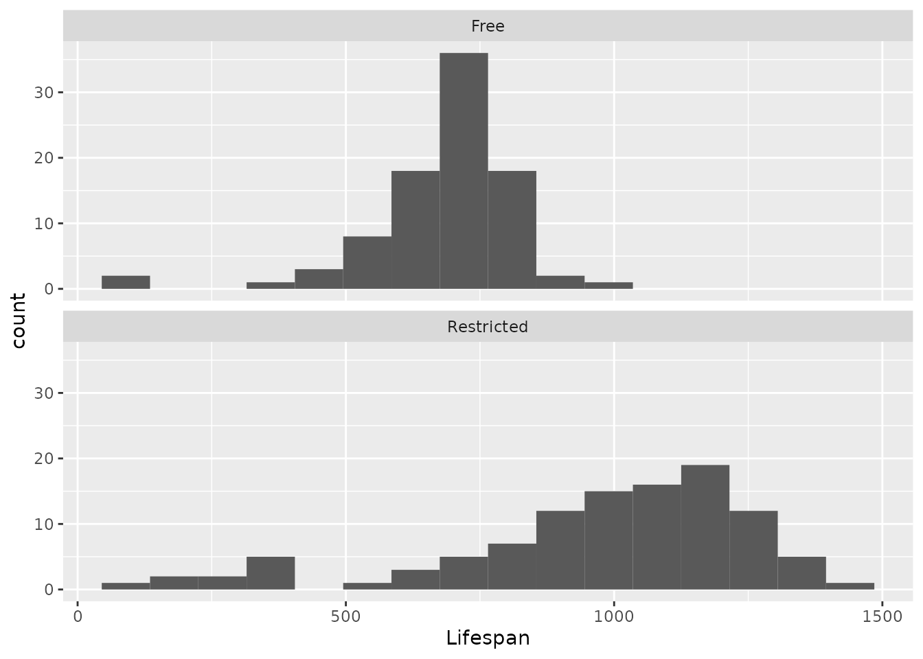

Exercise 3.4 First, let’s describe what we can see from the histograms (you may also try out other bin widths for the histograms as you like).

1. Describe the shape of the two distributions. Be sure to note the number of modes, any skewness, and whether there may be any outliers in either group.
2. Compare the two distributions. Be sure to note whether there seem to be any differences in central tendency or variability between the two groups.

3.3.2.2 Boxplots

We’ve also seen some examples of boxplots as useful visual summaries of data. The “box” of the boxplot encloses the “inter-quartile range” (IQR), that is, the middle 50% of the data that falls between the 25th and 75th percentiles. The line in the middle of the box shows where the median is. Boxplots are easy to produce in R by using geom_boxplot instead of geom_histogram:

rats %>%
    ggplot(aes(x=Lifespan, y=Diet)) +
    geom_boxplot()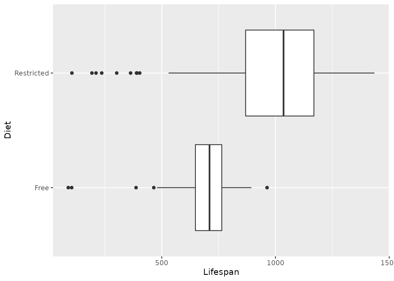

Exercise 3.5 Compare the boxplots and histograms we just made.

1. What sorts of things seem easier to do with the boxplots as opposed to histograms? Think about what features of the data might be easier to see with a boxplot and what comparisons might be easier to make using a boxplot.
2. Do you lose anything by using a boxplot instead of a histogram? Are there any important features of the data that are harder to see in the boxplot?

3.3.3 Summarizing the data numerically

Finally, let’s use R to get a numerical summary of the lifespans of the rats under the two diets. In the first part of the session, we focused on the mean and standard deviation (and variance), but we have also seen that the median and inter-quartile range (IQR) can also be used as numerical summaries of central tendency and variability.

R can find the median and IQR for us:

rats %>%
    group_by(Diet) %>%
    summarize(Median = median(Lifespan), IQR = IQR(Lifespan))

## # A tibble: 2 × 3
##   Diet       Median   IQR
##   <chr>       <dbl> <dbl>
## 1 Free         710   116 
## 2 Restricted  1036.  300.

___ %>%
    group_by(___) %>%
    ___(Mean = ___, SD = ___)

These numerical summaries of central tendency and variability provide a concise description of the lifespans of rats under the two different diets. These descriptions help us address the research question: does a restricted diet have an effect on lifespan?